The fusion of cranial skull plates in utero, or early in life, will result in an abnormal skull shape, also called craniosynostosis; from Greek origin (“σύν” and “ὀστέον”), meaning a closure of the bone sutures. This condition is generally treated with surgery, but the planning and evaluation is based on subjective criteria which depend on the experience of the craniofacial surgery team. We have developed a modelling tool to assess whether the skull shape can be recognized by a data-driven analysis similar to a bottom-up machine learning algorithm, and we use this to quantify the outcome of surgery objectively. In this study, we evaluated five scaphocephaly, six trigonocephaly, two brachycephaly and two plagiocephaly patients both preoperatively and postoperatively. Based on the kurtosis of the curvature distributions, we were able to classify the different types of craniosynostosis, and to quantitatively evaluate the postoperative results as being closer to a normal skull shape. In conclusion, we were able to design an algorithm automatically recognizing the type of craniosynostosis and quantitatively evaluating the surgical results as being closer or further away from a normal skull.
craniosynostosis, modelling, machine learning, skull growth, skull shape, surgical evaluation
Craniosynostosis is a condition in which one or multiple skull sutures fuse prematurely in infants [1], the shape of the skull depending on which suture is closed [2]. Surgery can correct the skull shape and relieve excess intracranial pressure [3]. Since each case is unique, multiple surgical approaches may be possible for a given patient. Therefore, the surgical team has a multitude of choices for a specific patient and decides on experience. There are currently no tools allowing a quantitative assessment of the severity of the deformation, or the surgical results.
Our overarching goal is to develop a system capable of predicting the outcomes of specific surgical approaches and provide a quantitative assessment of the performance of a respective approach. In our previous work, we have proposed a predictive model that allows craniofacial surgeons to perform virtual surgery on a patient’s head model, and subsequently simulate the postoperative head development of the model to qualitatively predict the surgical outcome. In the present paper, we describe a statistical model that can quantitatively measure the extent of deformity in skulls with craniosynostosis, using healthy skulls as a comparison, permitting a quantitative evaluation of a surgical approach by comparing the results of preoperative and postoperative skull shapes, allowing the selection of the optimal surgical approach.
Surface curvature estimation has been applied extensively in statistical shape analysis, as it provides dependable recognition of geometric characteristics [1]. With the introduction of 3D modelling in the medical field, curvature estimation has been commonly used in medical image registration [4], human structure modelling [5], and image segmentation [6]. Here, curvature estimation was used to classify different types of skull shape, into types of craniosynostosis.
We used previously acquired CT-scan from infants needing them for clinical reasons [7] with Research Ethics Board from Western University approval, which were then modelled as explained in Figure 1. All the results were plotted onto a two-dimensional figure with respect to two parameters, which we believed would most accurately depict skull shape. The first parameter is the Cranial Index ( ), which is a traditional clinical method used to evaluate a skull shape [8]. The second parameter is the summarization of a curvature distribution, which characterizes the local variance of the skull. Since the cranial index is a constant for each head scan, the key focus of our modelling was to investigate a proper way to summarize the curvature distribution. A set of training data, which includes typical cases from each type of craniosynostosis, was carefully selected to determine the best solution to differentiate curvature distributions among the types. Within the procedures, there are three steps (indicated by
  ) that could influence our final result. We proposed several options to implement each of the steps. With more data trained, we will adjust our simplification method
  , skull normalization
  , and the way to explain the curvature distribution
  , in order to make the result patterns as obvious as possible. More details for each step will be elaborated in the following sections.
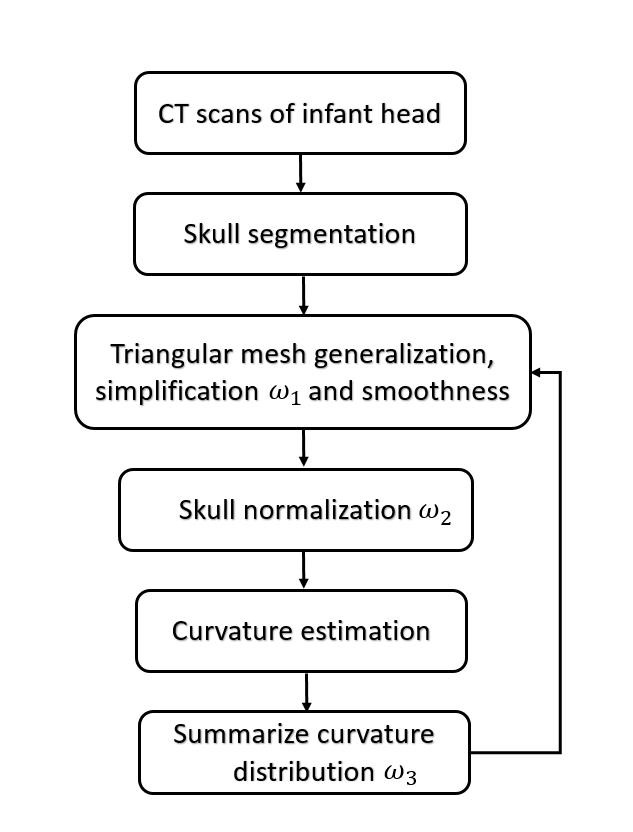
Figure 1. This is the flow chart of our statistical modelling, where are be adapted while more input data are involved in the training.
CT scans of craniosynostosis patients (archived using DICOM format) were retrospectively collected from our university hospital database to form our experimental group. We used previously acquired CT-scan from infants needing them for clinical reasons with Research Ethics Board from Western University approval [9]. The age of diagnosis of craniosynostosis ranged from shortly after birth to one-year-old, with cases between the years 2003–2012 included in our study. CT scans with voxel size larger than 0.4mm × 0.4mm × 2.0mm were excluded. As our gold standard, a set of CT images from a healthy 3-week-old baby was used as the basis of comparison. For the purpose of our study, we considered patients with scaphocephaly, trigonocephaly, brachycephaly and plagiocephaly to be abnormal. The final experimental group was comprised of five scaphocephaly, six trigonocephaly, two brachycephaly and two plagiocephaly patients.
In forming the training and test data sets, only preoperative head scans were used. Our training data consisted of two scaphocephaly cases, one trigonocephaly case, and two brachycephaly cases, which were carefully selected in order to best capture the shape features of the respective types of craniosynostoses. The remaining data formed our test data, which was used to validate our trained system.
Skull Segmentation and Surface Generation
In order to obtain a 3D representation of the skull shapes, we segmented each set of our CT images using Amira (Amira 5 User’s Guide - https://www.fei.com/software/amira-for-neuroscience/), a software tool that allows visualization and manipulation of images in three-dimensions. With the voxel labeling method in Amira, we labeled image intensities greater than 100 Hounsfield Unit (HU) as cranial bones. Cranial bones typically associated with surgical correction are membranous bones, which include the left/right frontal bones, left/right parietal bones, planum occipitale, and the flat portion of the temporal bone. Therefore, the remaining bone structures that have been labelled in the segmentation view were unselected. We stopped labelling the left/right frontal bones when the left/right orbital cavity started to be visible, and we erased the portion of temporal bones, in which the structure is more complicated than a curved plane. The planum occipital (the squama portion of occipital bone) contributed to our skull shape until the foramen magnum.
With the desired skull structures labelled, we proceeded to construct the surface outline of the skull shape. We used the existing weights method from the surface generation tools in Amira to extract two-layered skull shapes with triangular meshes. One layer represented the outer surface of the skull (in contact with skin), while the other layer indicated the inner surface that encloses the brain. In order to reduce the time required in further analyses, while still preserving enough detail of the shape, a fast but constrained simplification method (the parameter distance was set to 3) supplied in Amira was adopted.
Curvature estimation for discrete surfaces depends on the construction of vertices and faces that compose the surface. Therefore, we designed four methods to acquire the simplified skulls in order to determine the best solution for the following analysis. The first method is to continually simplify the skull until the number of faces of the mesh ceases to decrease any further. The second method is to simplify all the skulls to a certain number of faces (we selected 50000 faces). The third method is to halve the total number of triangular faces by four times for each skull. The final approach is to set the number of vertices of the skull meshes of a specific type at the same level (±500). Surface smoothing was applied subsequently to attenuate disturbances resulting from simplification. For smoothing parameters, we assigned 0.6 for diffuse factor and 20 for iteration times.
Skull Volume Normalization
It is important to keep in mind the variability that exists in skull shape between individuals. Moreover, even if two babies have similar skull shapes, they could still have different intracranial volumes since head circumference varies at birth. This would lead to different curvature distributions between the individuals, where the baby with the larger volume will tend to have a lower curvature distribution. Thus, it is important to normalize intracranial volume between individuals. This can be accomplished by taking two similar skulls, and uniformly scaling one skull so that its width is the same as the other skull. This would result in similar intracranial volumes between the two skulls, with a similar range of curvature values. To this end, the skull width and length must be calculated for each case, where skull length is for the calculation of cranial index.
We developed an algorithm to semi-automatically calculate the skull width and length, using the healthy skull of the 3-week-old infant as a reference. The algorithm must recognize the orientation of the skull model, so we chose to manually define the sagittal plane of the skull. At least three points are required to define a plane, and we chose the center of the skull, along with two other locations that could be manually selected on the skull mesh.
The centroid is calculated with the weighted average of face locations on the mesh:
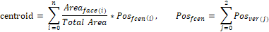
where n is the total number of faces in a skull model,  is area of the ith face,
  is the centroid of this ith triangular face, and
  is the position of jth vertex from a triangular face.
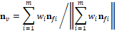
The second point we selected is at the bottom of the frontal suture of our model, which should be close to the nasion (the intersection of the frontal bone and the two nasal bones). The third point we selected was at the external occipital protuberance, which is a protruding point located in the middle of the squamous part of occipital bones. With these 3 points, the normal of the sagittal plane can be calculated with the following equation:

Where  is the vector pointing from centroid to the second point,
  is the vector pointing from centroid to the third point.
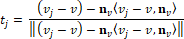
With the normal of the sagittal plane, we can find another line that goes in the same direction through the centroid of the skull, intersecting with both the left and right side of the skull. We took the distance between these two intersected points as the skull width. To calculate the skull length, we first explored the farthest position of the skull mesh that is within the sagittal plane from the center point. We determined whether a vertex is in the sagittal plane with the following equation:

Where  is the vector from the centroid of skull to the center of ith face, and the value of the tolerance is 0.0001. The second investigation followed is to find another vertex in this sagittal plane that has the longest distance with previous location. The distance between these two locations is defined as the skull length.
Curvature Estimation for Discrete Surface Meshes
We selected a curvature estimation algorithm developed by Dong and Wang (2005) in our evaluating system [7]. Consider a surface mesh G = (V, F), where V represents a set of vertices in the surface and F defines the triangular faces that link those vertices together. For each triangular face  , it is easy to obtain the unit normal vector
  . To find the tangent plane of a vertex in the mesh, Dong and Wang took advantage of the faces in the vicinity of this vertex, which are one-ring faces around the vertex [7]. Let
 be a vertex on the mesh G, and
  denotes faces in the one-ring neighbourhood of v. The normal vertex
  of vertex
  can be averaged by weighted normal vectors of faces that are in the one-ring neighbourhood of
  :
:

Where  is the unit normal vector of face
 and
and  is the coordinate of the centroid of face
 . The method to define the weight of face
  was proposed by Chen and Wu (2004) [16].
For each vertex on a surface mesh, there are a series of vertices
  surrounding it in the area of one-ring neighbourhood. Let assume the distance between
  and is small enough, and thus we can obtain:
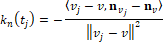
Where  indicate the tangent vector of the curve that forms and . We can interpret this tangent vector as the projection of vector
  on the tangent plane of . Therefore,
Dong and Wang introduced the least square method from Chen and Schmitt to estimate principal curvatures [7,10]. It is known that normal curvatures of a vertex has such relation 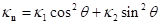 according to Euler’s equation, where
  and
and  are maximum and minimum curvatures at , and
  is the angle between and
  . Since the direction of and are unknown, Dong and Wang proposed to select an arbitrary coordinate system
  on the tangent plane [7]. Let
  denote the angle between the direction of and
  , and
, and  denote the angle between the direction of
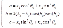
  and . Therefore, the Euler formula can be converted to:

Where the constants a, b, c can be represented with respect to , and :
If we use the maximum normal curvature  among
among  to build the coordinated system , where the direction of is , it is easy to obtain
  . Therefore, b and c can be estimated as:
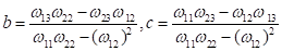
Where:
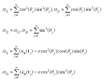
Dong and Wang also provided the relationship between the constants and curvatures:
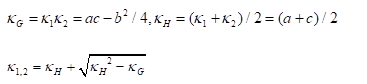
Where  is the Gaussian curvature,
  is the Mean curvature, and
  are the Principal curvatures.
In summary, the above algorithm for calculating the Principal curvatures of a vertex utilized one-ring neighbourhood of faces and vertices. Alternatively, it is implementable to involve k-ring neighbourhood in this algorithm if necessary. In our work, we choose two-ring neighbourhood, trying to smooth local noises during mesh simplification meanwhile to keep  (distance between and ) as small as possible for accuracy. In addition, we would only take use of the maximum curvature in our evaluation tool.
Curvature Distribution for One Skull Shape
A curvature value obtained from the aforementioned algorithm is only a representation for one vertex on a surface mesh, since it only depicts local changes. Each skull mesh is composed of a large amount of vertices, and we therefore obtained a series of curvature values for each skull shape.
We used curvature distribution to render the set of curvature values on a 2D figure, where the x-axis represents curvature values and the y-axis indicates the percentage of vertices on a mesh that falls onto the same curvature value. Smooth objects more spherical in shape should display a narrow and tall distribution, whereas objects ellipsoidal in shape should have a shorter but wider distribution. We expected that similar skull shapes on the same scale should display similar distributions, and that we would be able to distinguish the different types of skull shapes by their patterns of curvature distribution. However, for discretized manifolds with noises, it is hard to obtain exactly same curvature values for two vertices. Therefore, we need to divide the range of this set of vertices into segments.
Since the shape of a normalized skull is more ellipsoid in shape, the range of curvatures can be decided. We set the range of curvature values to be (0, 0.1), then further divided this range into small bins, each of which should have the same value (e.g. bin=0.001 or 0.005). As a result, each bin represents a smaller range of curvature values within (0, 0.1). The curvature value of a vertex that falls into any bin should contribute to the y-axis (percentage of vertices) of the according bin.
In order to study the pattern of different skull shapes, we designed the statistical model to use two parameters as contributions. The first parameter used was the cranial index, which roughly describes the scale of the skull volume. The second parameter was the curvature distribution of a skull. However, curvature distribution is a curve that represents how curvature values of a mesh behave within a certain range, which means that the pattern of curvature distribution will vary depending on different types of shape. Thus, a method of summarizing the pattern of curvature distribution into one variable was needed.
In statistics, moment is a common way to quantify the shape of a distribution curve or a set of points. There are four significant moments: the mean (1st moment), variance (2nd moment), skewness (3rd moment) and kurtosis (4th moment) respectively.
The kurtosis is defined as normalized fourth moment, and measures the weight of the tail for a distribution:
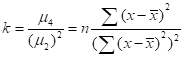
Where  is the variance and
  is the fourth moment. If the value of k is 3, the distribution is a normal distribution. If the value of k is greater than 3, the distribution tends to have long and fat tails, whereas values lower than 3 will have distributions with short tails. Considering the geometrical meanings of significant moments, we decided to utilize kurtosis to measure the curvature distribution.
System Development with Training Data
In this section, we will demonstrate how mesh simplifications, skull normalization and the bin values of curvature distribution affect the performance of our system. For each feature, we will represent the results with all possible approaches we implemented, while the other features were fixed.
Mesh Simplifications
Figures 2 to 5 represent the measurements of skull shapes with four different approaches of mesh simplification. All other parameters were kept constant. The iteration value for surface smoothness was set to 20, all the skulls were normalized, and the bin value was 0.005. We represented a skull shape with both cranial index and kurtosis (in log) of its curvature distribution.
Figure 2 indicates various skull shapes, which were all composed of 50000 triangular faces. The black dot is from a healthy baby, the two green dots indicate scaphocephaly cases, the blue dots represent two brachycephaly cases, and the red dot is from a trigonocephaly patient. From the x-axis, we can see that scaphocephaly patients have lower values than the other cases, the trigonocephaly skull was closer to a healthy shape, and the values of the two brachycephaly cases were relatively higher than the others. While we expected that the distribution of kurtosis values could differentiate the different types of craniosynostosis, this was not the case. One brachycephaly patient was at the same level as the control patient, and one scaphocephaly case had the highest value while the other scaphocephaly case had the lowest.
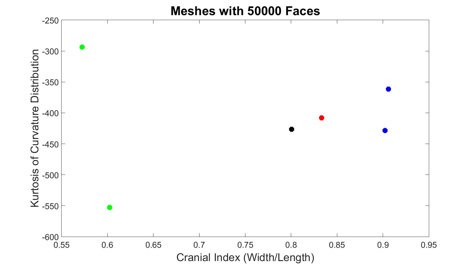
Figure 2. Results from training data, which the number of faces of each surface mesh is 50000. The black dot is the normal skull, the green dots are the scaphocephaly, the red dots are the trigonocephaly, the blue dots are the anterior plagiocephaly.
Figure 3 represents skull meshes that were simplified until the number of faces ceased to change. While x-axis values were the same as previous, the values of kurtosis were quite different. The kurtosis of the normal skull was distinct from pathological cases. However, one value of scaphocephaly was higher than the trigonocephaly and brachycephaly patients, while the kurtosis value of the other scaphocephaly case was the lowest. Therefore, this method was also unable to classify the types of skull shapes.
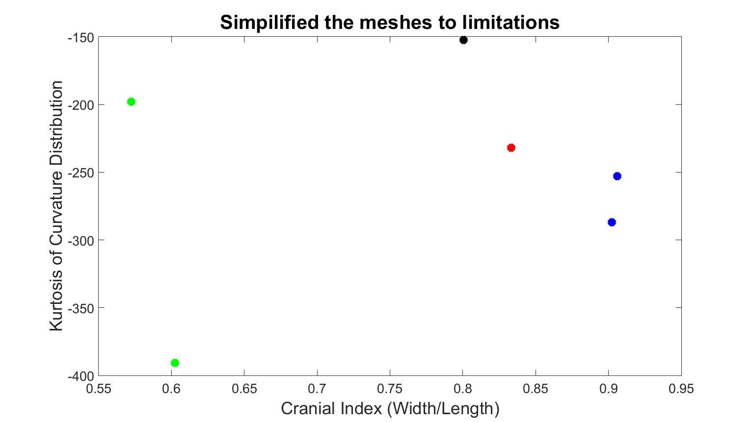
Figure 3. Quantified results with the second mesh simplification method, which reduces the number of faces to the limitations. The black dot is the normal skull, the green dots are the scaphocephaly, the red dots are the trigonocephaly, the blue dots are the anterior plagiocephaly.
Figure 4 displays skull meshes where the number of faces was all halved by four times. Figure 5 shows the skull shapes with similar numbers of vertices. Under both simplification methods, the different types of craniosynostosis were able to be differentiated in similar patterns. The healthy skull had the lowest kurtosis value, the trigonocephaly skull had a greater value, the brachycephaly patients had even greater value, and the scaphocephaly cases had the highest value. The values of scaphocephaly cases deviated furthest from the control case, which corresponds to the fact that scaphocephaly skulls are the most deformed. In addition, the value of the trigonocephaly case was closest to the control case while the shape of this type of skull was similar to normal shape only except the forehead and the cranial index was in the same range as normal.
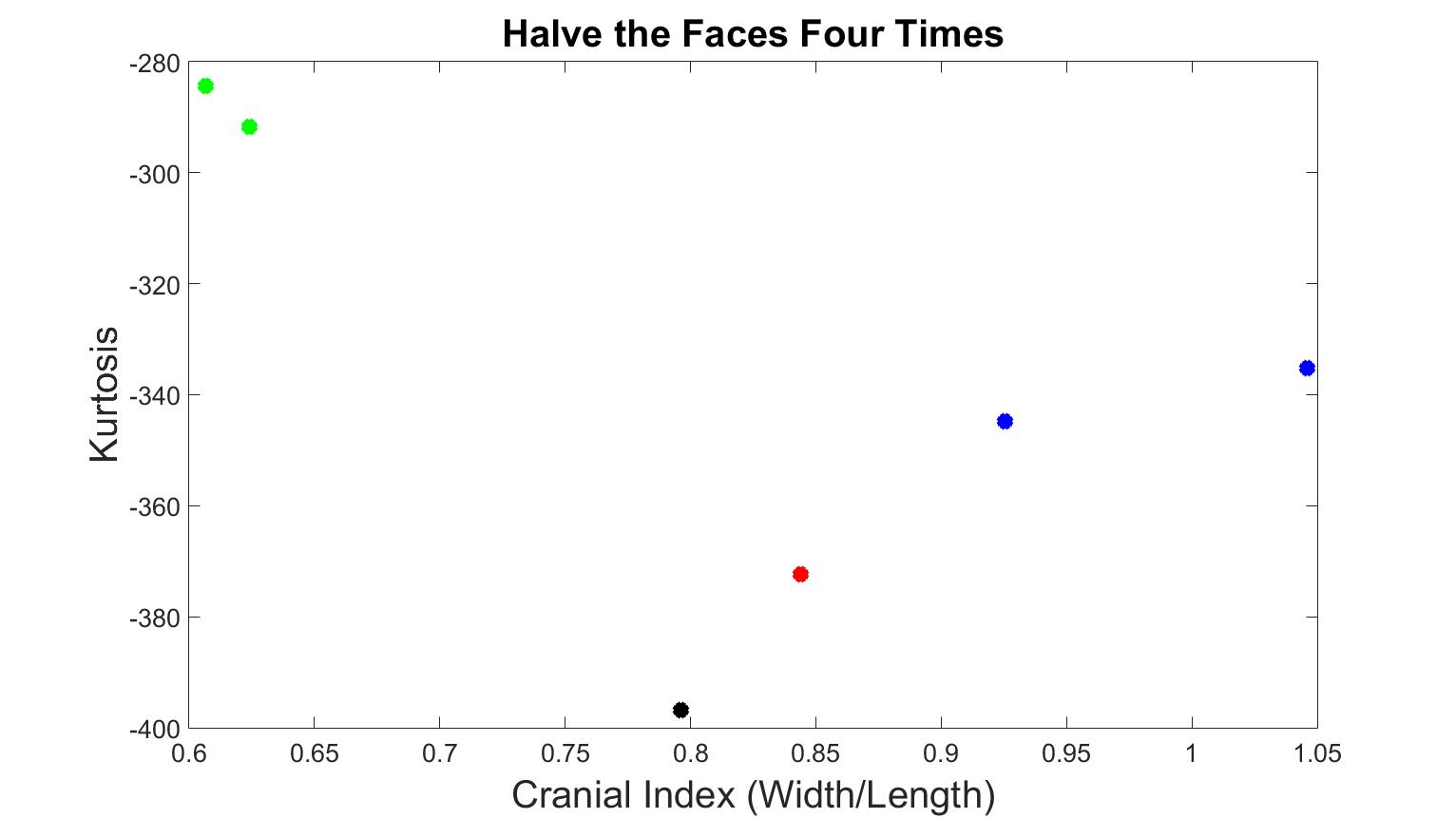
Figure 4. Kurtosis vs cranial index with different skull shapes, which number of faces were halved four times. The black dot is the normal skull, the green dots are the scaphocephaly, the red dots are the trigonocephaly, the blue dots are the anterior plagiocephaly.
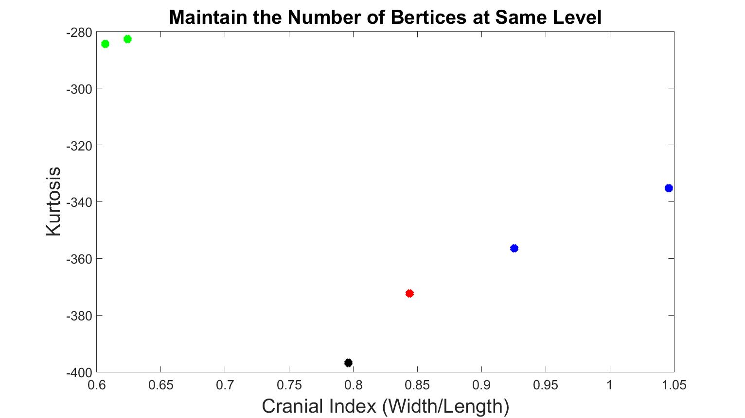
Figure 5. Kurtosis vs cranial index with different skull shapes, which number of vertices were at the same level. The black dot is the normal skull, the green dots are the scaphocephaly, the red dots are the trigonocephaly, the blue dots are the anterior plagiocephaly.
Since both methods were effective, we decided to combine them. First, for all the skull shapes, the number of faces was halved four times. On the basis of this step, for each type of craniosynostosis, we selected the skull that had the smallest number of vertices, and tuned the number of vertices of the other skulls to the same level, allowing ±500 difference depending on the complexity of the skull shape.
Skull Normalization
With a selected mesh simplification method, we tested whether skull normalization was necessary or not. With the optimized simplification method and bin = 0.005, we inputted the training data into our system without normalization, as displayed in Figure 6. The kurtosis value of trigonocephaly was higher than the values of the brachycephaly cases, and the value of one scaphocephaly case was at the same level as the trigonocephaly case. This demonstrates that without skull normalization, the distinct shapes of scaphocephaly and trigonocephaly cannot be differentiated. In addition, the kurtosis value of trigonocephaly was unexpectedly greater than brachycephaly. As a result, we decided to continue with skull normalization in the following experiments.
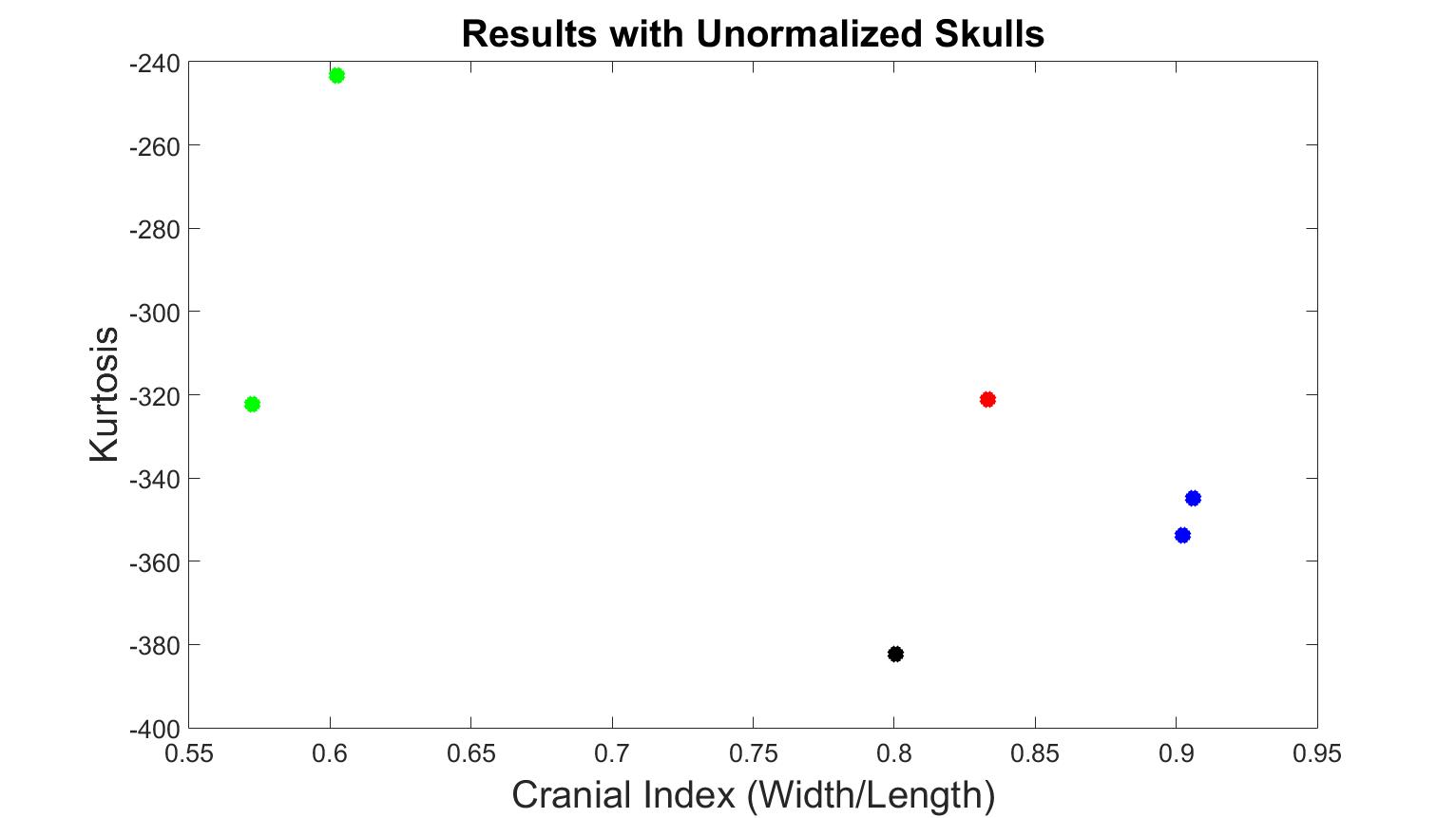
Figure 6. Kurtosis vs cranial index with different skull shapes without normalization. The black dot is the normal skull, the green dots are the scaphocephaly, the red dots are the trigonocephaly, the blue dots are the anterior plagiocephaly.
The Bin Values
Next, we explored the optimal bin value that would best classify the types of skull shapes. We tested bin values from 0 to 0.01, in 0.0005 increments.
The results of 0.0005, 0.001, and 0.01 bin values are displayed in Figures 7 to 9. At these bin values, the different types of craniosynostosis could not be differentiated from normal (the values of brachycephaly patients all overlapped with the values of trigonocephaly cases).
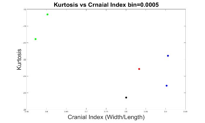
Figure 7. The measurements of skull shapes with bin=0.0005.
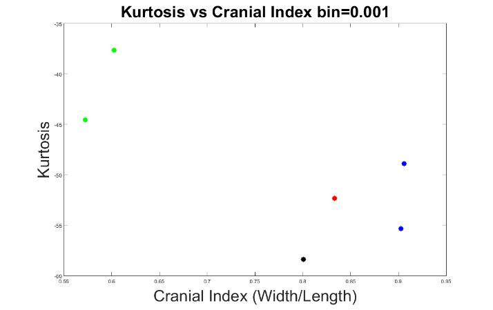
Figure 8. The measurements of skull shapes with bin=0.001.
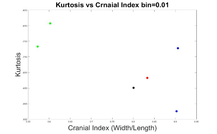
Figure 9. The measurements of skull shapes with bin=0.01.
Figures 10 to 13 display the results with other bin values (0.004, 0.005, 0.006 and 0.008). With these values, our system was able to demonstrate the types of craniosynostosis well, from which we could see that both Figure 11 and 13 best differentiate the craniosynostosis types, but indicated with different patterns, where the kurtosis values of brachycephaly cases were higher than the trigonocephaly case in Figure 11, which pattern was inverted in Figure 13. Since we hope that with a closer cranial index to normal case, the kurtosis value should be closer to normal. As a result, we preferred bin = 0.005 to be the most appropriate value.
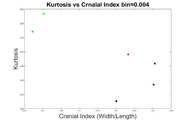
Figure 10. The measurements of skull shapes with bin=0.004.
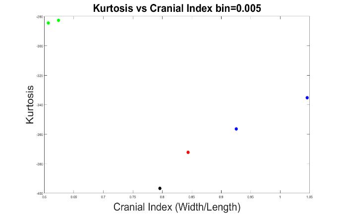
Figure 11. The measurements of skull shapes with bin=0.005.
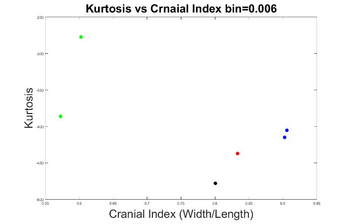
Figure 12. The measurements of skull shapes with bin=0.006.
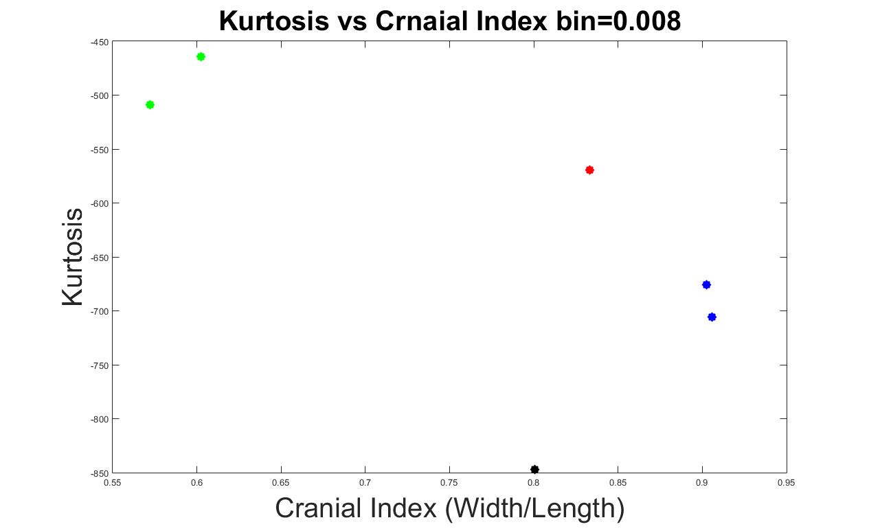
Figure 13. The measurements of skull shapes with bin=0.008.
System Testing
We added test data into our system to investigate its accuracy. As a comparison, we also provided the results with bin=0.008, which was previously a good indication between different types of craniosynostosis with our training data (as seen in previous section). In Figure 14 and 15, we added three scaphocephaly patients and four trigonocephaly cases, with bin values 0.005 and 0.008 respectively. As seen in Figure 15 (bin=0.008), the system was able to accurately characterize the types of craniosynostosis except for two scaphocephaly cases, which were overlapped with the values of trigonocephaly cases. Again, although the trigonocephaly cases obtained very similar kurtosis values, they were still unexpected higher than brachycephaly cases. A bin value of 0.005 was confirmed to be optimal for our evaluating system since the skull shapes dispersed in the figure in a way such that the further a cranial index deviated from the control case, the further the corresponding kurtosis value deviated from the value of normal.
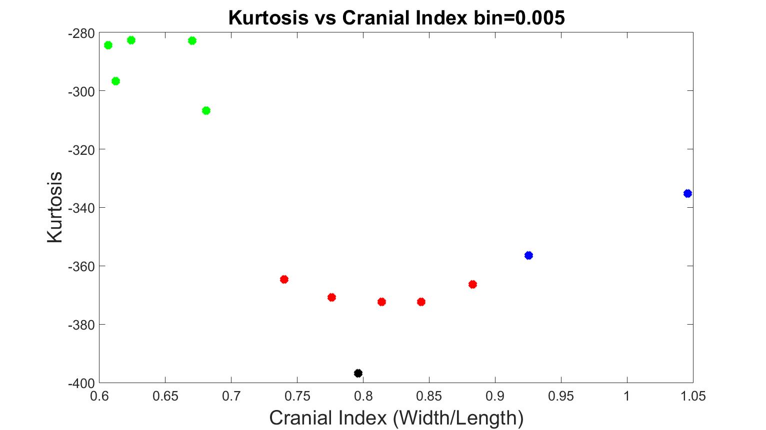
Figure 14. The measurements of skull shapes from test data with bin=0.005.
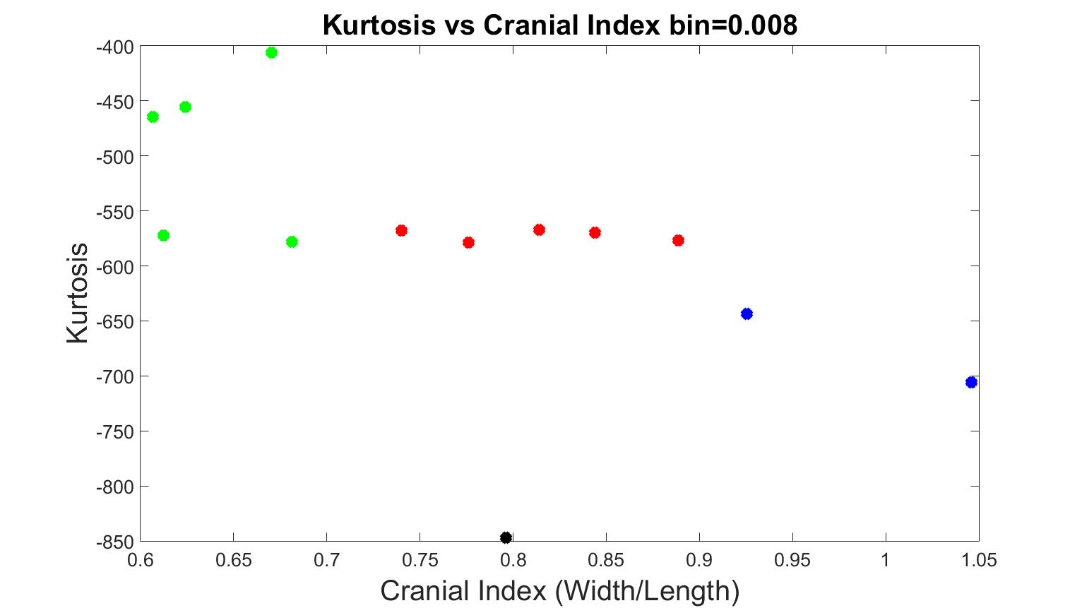
Figure 15. The measurements of skull shapes from test data with bin=0.008.
With the confirmation of our evaluating system with bin=0.005, we further added one atypical trigonocephaly and two anterior-plagiocephaly cases (Figure 16). We also provided an aerial view of an atypical trigonocephaly skull in Figure 17, next to a typical trigonocephaly skull. A typical trigonocephaly patient should have a triangular forehead (Figure 17), whereas the forehead of the skull at the right side looks normal. We can only see the deformity from the side view of this skull in Figure 18, and neurosurgeon diagnosed this skull as a mild trigonocephaly. Looking back to Figure 16, the cranial index of this patient was 0.812, which was considered in the normal range, and the kurtosis value was lower than the values of typical trigonocephaly cases. Therefore, our evaluating system indicated this case as a mild trigonocephaly case, which matched the truth.
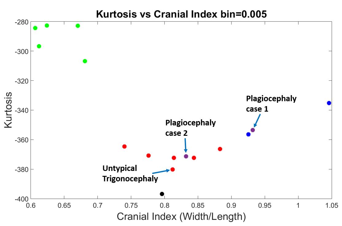
Figure 16. Best results with a bin value of 0.005. The black dot is the normal skull, the green dots are the scaphocephaly, the red dots are the trigonocephaly (the one with the arrow is a bit less typical when observed clinically by an expert), the blue dots are the anterior plagiocephaly.
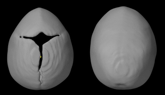
Figure 17. Top view of trigonocephaly skulls, the left one is a typical shape and the right one is the untypical case shown with an arrow in Figure 16. While the metopic suture is closed, the skull is less “pointy”.
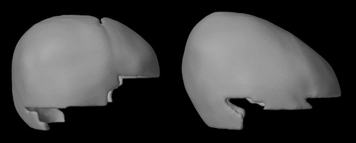
Figure 18. Side view of trigonocephaly skulls, the left one is a typical shape and the right one is the untypical case shown with an arrow in Figure 16. While only the metopic suture is closed, the skull is elongated and the parietal bone is higher than expected.
The purple dot, which was close to one of the brachycephaly skull shapes (blue dots), was denoted as “plagiocephaly case one”. The right side of Figure 19 showed the top view of this skull shape, whereas the left side was from the brachycephaly patient (blue dot) that was very close to this plagiocephaly case in Figure 16. We can see from Figure 19 that both skulls had similar shapes, which were both flat and short. In addition, these two skulls had similar cranial index values indicated in Figure 16, and is therefore their kurtosis values were anticipated to be close.
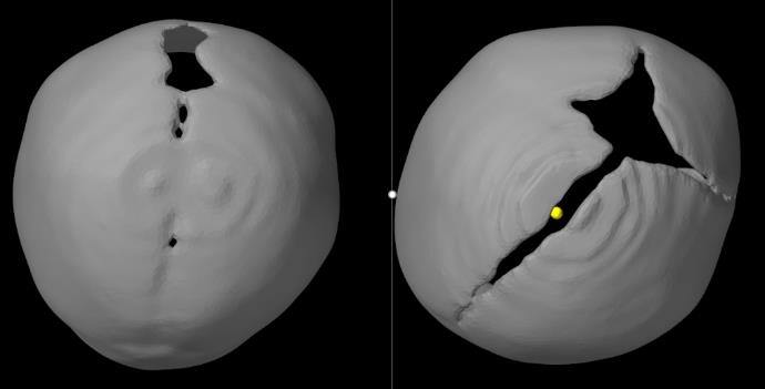
Figure 19. Comparison of skull shapes from top view between a brachycephaly (left: bilateral coronal synostosis – also seen as bilateral anterior plagiocephaly) and a left plagiocephaly patient (right image).
The second plagiocepha2021 Copyright OAT. All rights reserv trigonocephaly region, surrounded by red dots in Figure 16. We provided the top view of this skull shape in the right side of Figure 20, and the top view of the first plagiocephaly skull shape at the left side. As comparison, we can see the level of deformity of this second plagiocephaly skull was much less severe than the first one, and the value of cranial index was 0.83 that was close to our normal case. As a result, it is predictable that the kurtosis value of this patient was lower than the first plagiocephaly case and much closer to the normal patient.
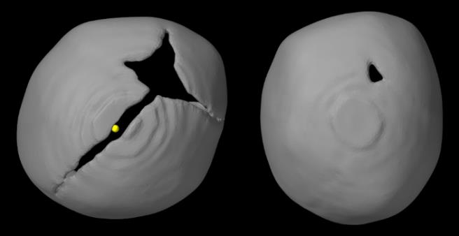
Figure 20. Comparison of skull shapes from top view, between 2 left anterior plagiocephaly to show how variations can occur even with the same suture being closed.
Curvature is an intrinsic feature that describes the local shape of a surface, and therefore, calculating the curvature values of a skull is the key procedure in our evaluation system. Surface mesh, which is composed of triangular faces and vertices, was adopted to generate each skull, and each vertex has a curvature value according to its neighbourhood of vertices and faces. We used a statistical method called kurtosis to summarize all the curvature values of a skull mesh into one number, which can be outputted with the cranial index of a skull. There were several steps in our algorithms, which could affect the curvature values, such as the method for simplifying the skull shape, the size of the skull shape, and the method for representing a curvature distribution. We selected several skull shapes from different types of craniosynostosis as training data, which were repeatedly inputted into our evaluating system with different algorithms in order to determine the best way to classify the different types of shapes.
Cohen and Maclean categorized skull shapes into four types on the basis of CI: dolichocephaly (CI ≤ 75.9), mesocephaly (CI between 76.0 and 80.9), brachycephaly (CI between 81.0 to 85.4), and hyper-brachycephaly (CI ≥ 85.5) [11]. A typical skull shape for scaphocephaly would most likely be dolichocephaly, and the CI of a typical brachycephaly head ought to be higher than 85.5. This validated our algorithm to calculate CI from Figure 21, where the CI’s of all the scaphocephaly cases were lower than 0.7, and the CI’s of the two brachycephaly cases were higher than 0.9.
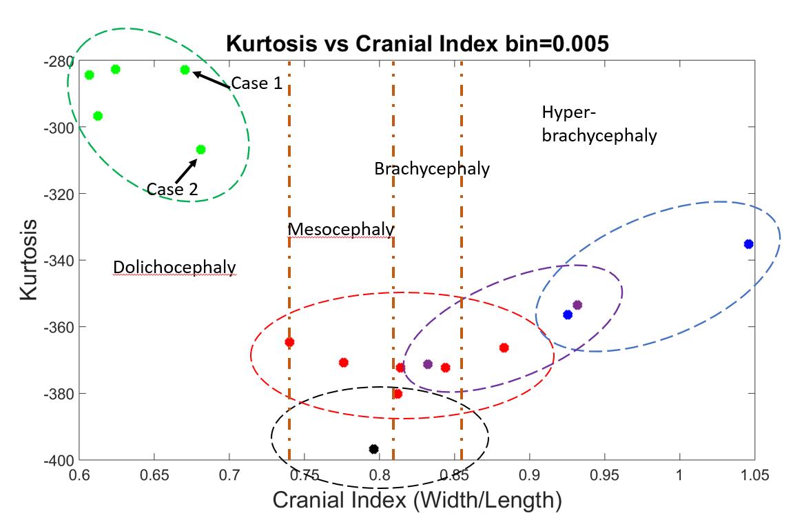
Figure 21. An indication of expected areas of shape results for each type of skull shapes. Dolichocephaly, mesocephaly, brachycephaly and hyper-brachycephaly were separated by yellow-vertical-dashed lines.
On the other hand, not all shapes categorized as dolichocephaly, brachycephaly, or hyper-brachycephaly are pathological. In a previous study, 35 Polish children (aged 4-6 months) and 53 Polish children (aged 7-12 months) diagnosed as having normal head shapes were found to have an average CI of 81.45±7.98 and 83.15±7.98, respectively [8]. According to the study, although mesocephaly is the dominant head shape among children with normal head development, other head types present as well, especially brachycephaly [8]. Similar results were also found in a cohort of infants from the United States [12]. Wolański et al. [13] found that the average CI for infants between the age of 0 to 6 months is 83.75±7.25, whereas Dekaban concluded the average CI for infants within 12 months is 78.36 [13,15]. In addition, some skull shapes may exhibit a combination of several different features, such as a trigonocephaly patient with brachycephaly head shape (the red dot in Figure 21 with CI of 0.88). As a consequence, for the CI values for each type of skull shape, we would expect an area on our 2D output figure distributed by diverse cases of one type of craniosynostosis, which reasonably overlaps with areas of other types (dashed ellipses in Figure 21). With more data added, we expect each area will be enlarged.
Although we only had one normal case in our database, this normal head shape was a mesocephaly. As the middle point among all the CI values, we considered this normal head to be our standard head shape. If any pathological skull shape was restored back to this shape, we regarded the associated surgery to be effective for this patient. We would expect that other normal shapes would be distributed within the black dashed circle shown in Figure 21.
The kurtosis values in our research were interpreted as the summary of a head’s local shapes, and the extent of deformity of a skull shape. Generally, we assumed that the further the CI value deviated from our normal case, the greater the extent of deformity in the skull. The results in Figure 21 validated our assumption, and also matches research from Ruiz-Correa et al. [14]. In their study, which measured the severity of scaphocephaly heads, the CI was found to have a positive linear correlation with their severity measurement of scaphocephaly head shapes [14]. Therefore, the overlapped regions could also be explained by the fact that some skull shapes might be very similar even if they belong to different types of craniosynostosis, or the same level of deformity but with different head shape.
However, the kurtosis values could also fluctuate due to certain factors. Consider two scaphocephaly cases as an example, which are indicated by case 1 and 2 in Figure 21. The CI’s of these two cases were very close, but the kurtosis values had a gap in between. We provided the curvature distributions of these two skulls in Figure 22 with a color map of curvature, showing from blue as 0 to red as higher than 0.1. From an aerial view, case 1 had a short and wide forehead, and the skull width narrowed towards the posterior end, whereas the width of case 2 was essentially constant across the skull. Therefore, the difference in local shapes could result in the discrepancy of kurtosis values, even though the CI values are the same. In addition, case 1 had more high values of curvature (indicated by more yellow and red regions) than case 2, especially along the edges of open areas and along the midline. We excluded curvature values higher than 0.1 from our shape quantification algorithm. As a result, less curvature values in case 1 contributed to the skull shape evaluation, which can explain the higher than expected kurtosis values.
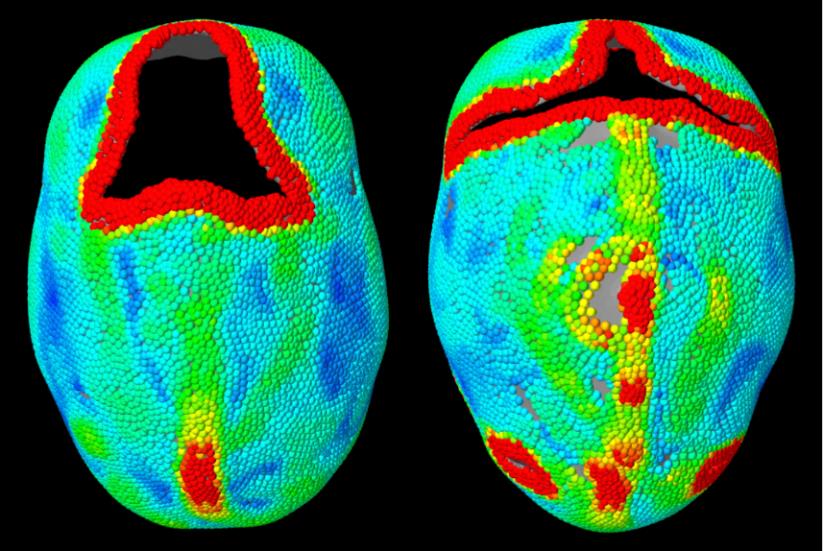
Figure 22. A comparison of local shapes between two scaphocephaly patients (right is case 1 and left is case 2), indicated by color map of curvature values showing from low to high (blue as 0 to red).
Our system can be considered stable if the inputted skulls have small open areas or relative short edges, though this cannot be ensured in many cases – especially for postoperative skulls.
Future studies should attempt to determine a method to smoothly fill the open area of a skull in order to render the result as accurately as possible. Another step would be to increase the amount of clinical data used as training data to further tune our evaluating algorithms, resulting we believe in an expansion of the region in the graph for each craniosynostosis type. We also hope to be able to effectively apply this algorithm to evaluate surgeries by comparing preoperative and postoperative skull shapes to normal cases, and determine how far the postoperative skull shape shifted towards the ideal normal shape.
We developed an algorithm able to quantify skull shape, allowing craniofacial surgical teams to not only qualitatively evaluate an abnormal skull, but also to quantitatively evaluate the degree of postoperative improvement compared to the preoperative skull shape.
We evaluated the extent of skull deformity for each common type of craniosynostosis in a way where the further a cranial index value deviates from the control patient, the further its kurtosis deviates from the normal. From another perspective, with similar cranial index and the same type of shape, the kurtosis values are varied by the local shapes and the length of skull edges (caused by open areas). With this evaluating algorithm, we can evaluate a craniosynostosis surgery by inputting the skull measurements of a patient from different periods in that patient’s life. Ideally, an effective surgery should produce postoperative skull shapes with corresponding kurtosis values and/or cranial indices that shift closer and closer to the gold standard normal shape.
The research was done with ethics approval. All the figures are our own.
Jing Jin: Modeling and running of the data, preparation of the manuscript; Roy Eagleson: Supervision of the modeling as well as design of the experiment, review of manuscript; Sandrine de Ribaupierre: General idea for research. Design of the experiment, preparation of manuscript.
No competing interests to declare
Our project is supported by the Engage Grants from Natural Sciences and Engineering Research Council of Canada. Thank you to Marcus Lo for reviewing and formatting the manuscript.
- Johnson D, Wilkie AOM (2011) Craniosynostosis. Eur J Hum Genet, 19: 369–376.
- Aviv RI, Rodger E, Hall CM (2002) Craniosynostosis. Clinical Radiology, 57: 93–102.
- McCarthy JG, Glasberg SB, Cutting CB, Epstein FJ, Grayson BH et al., 1995. Twenty-year experience with early surgery for craniosynostosis: II. The craniofacial synostosis syndromes and pansynostosis--results and unsolved problems. Plast Reconstr Surg., 96: 284–295; discussion 296–298. [Crossref]
- Cui M. et al. (2007) A new image registration scheme based on curvature scale space curve matching. The Visual Computer, 23: 607–618.
- Santiesteban, Y., Sanchiz, J.M. & Sotoca, J.M., 2006. A Method for Detection and Modeling of the Human Spine Based on Principal Curvatures. Progress in Pattern Recognition, Image Analysis and Applications, 4225: 168–177.
- Zhang X. et al. (2008) 3D Mesh Segmentation Using Mean-Shifted Curvature. In F. Chen & B. Jüttler, eds. Advances in Geometric Modeling and Processing. pp. 465–474
- Dong C, Wang G (2005) Curvatures estimation on triangular mesh. Journal of Zhejiang University-Science A, 6: 128–136.
- Likus W, Bajor G, Gruszczyńska K, Baron J, Markowski J, et al., (2014) Cephalic index in the first three years of life: study of children with normal brain development based on computed tomography. ScientificWorldJournal, 2014, p.e502836 [Crossref]
- Mendoza CS, Safdar N, Okada K, Myers E, Rogers GF, et al., (2014) Personalized assessment of craniosynostosis via statistical shape modeling. Med Image Anal, 18: 635–646 [Crossref]
- Chen X, Schmitt F (1992) Intrinsic surface properties from surface triangulation. In Computer Vision—ECCV’92. Springer 739–743
- Cohen MM, MacLean RE (2000) Craniosynostosis: Diagnosis, Evaluation, and Management, Oxford University Press
- Hummel P, Fortado D (2005) Impacting infant head shapes. Adv Neonatal Care, 5:329–340. [Crossref]
- Wolański W, Larysz D, Gzik M, Kawlewska E et al., 2013. Modeling and biomechanical analysis of craniosynostosis correction with the use of finite element method. Int J Numer Method Biomed Eng, 29: 916–925 [Crossref]
- Ruiz-Correa S, Sze RW, Starr JR, Lin HT, Speltz ML et al., 2006. New scaphocephaly severity indices of sagittal craniosynostosis: A comparative study with cranial index quantifications. Cleft Palate Craniofac J, 43: 211–221 [Crossref]
- Dekaban AS (1977) Tables of cranial and orbital measurements, cranial volume, and derived indexes in males and females from 7 days to 20 years of age. Ann Neurol., 2:.485–491. [Crossref]
- Chen SG, Wu JY (2004) Estimating normal vectors and curvatures by centroid weights. Computer Aided Geometric Design, 21: 447–458.