Take a look at the Recent articles

Abstract

As a physiological index, energy expenditure (EE), is of great significance in sports rehabilitation and other fields. The traditional way to measure EE is time consuming and requires heavy equipment. Therefore, it is important to develop a fast and accurate method to predict EE. The surface electromyography (sEMG) is one of the most important parameters in estimating EE, however, it is often used in a single model, which leads to poor accuracy and stability. In this paper, the machine learning regression algorithm based on the decision tree model represented by the XGBoost and the neural network model represented by the long short memory term (LSTM) were applied to predict and evaluate EE. Finally, these models were fused, and the prediction results of various models were further improved by the fusion algorithm.

Keywords

energy expenditure prediction, EMG, model fusion, machine learning, time series prediction

Introduction

The concept of energy expenditure (EE) was first proposed by Italian physiologist DiPrampero in 1986 and was defined as maintaining basic metabolism and satisfying various physical activities (PAs) [1]. Previous studies have shown that the level of PAs is negatively associated with the risk of a range of chronic diseases [2,3].

In the field of rehabilitation, exoskeletons are widely used to assist people with disabilities in their activities of daily living and gait training. Individualised or personalised assistance requires an accurate EE estimation [4], which is used to assess the effect of the exoskeleton on the user's energy saving as well as the burden of the exoskeletal structure worn by the user. Moreover, for patients with bone injuries [5,6], stroke [7], and surgical patients, accurate assessment of EE during exercise and determination of the appropriate amount of exercise are crucial for reducing the sedentary nature of rehabilitation [8]. In addition, the accurate assessment of EE in athletes can help develop individualised training programs [9,10]. Finally, the concept of individualised diagnosis and treatment has recently been proposed [11-13].

Thus, the real-time measurement of EE is important for human health and safety. EE is the state of the body that can only be inferred, estimated, or measured using measurable signals (e.g. heart rate). There are three types of measurable signals related to EE. Type 1 is governed by the laws of physics, chemistry, and biology. This relationship is also known as a relationship based on physical principles [14-16]. Type 2 is governed, in part, by the laws of physics, chemistry, and biology. For example, one may determine whether a relationship is linear or quadratic. This relationship is called semi-empirical [14,15,17]. Type 3 is unknown in terms of physics, chemistry, and biology. This relationship is empirical [14,15,17] and can be predicted using statistics and machine learning. It is possible to combine two or three types of signals, which is also known as sensor fusion.

Different types of signals have advantages and disadvantages. Type 1 signals are more accurate, but invasive and non-online. Type 2 signals are online (thus facilitating effective monitoring, while humans maintain natural activities and remote monitoring) and are less intrusive or noninvasive but less accurate. Type 3 signals are the most accurate, unreliable, and least stable. The development of an accurate, online, non-invasive, and non-intrusive method remains an open problem. One direction for development is to explore new signals that may correlate with EE and be much easier to use than existing signals using wearable sensors. A more general approach for combining can be found in [18]. For example, acceleration and heart rate were found to accurately correlate with EE [19,20]. However, this approach is not applicable to sedentary or very slow movements. One method to address this shortcoming is to include an electromyogram to form a three-signal marker [21]. Another direction of development that is relevant to the multi-signal marker approach is to combine them by considering their significant contribution to the correlation to EE, for example, the weighted average combination. Indeed, the generation of EE by PAs always occurs in an environment in which many state variables are generated simultaneously to contribute to their correlation with EE.

Based on the signal categorisation for estimating the aforementioned EE, methods for estimating EE include approaches based on physiological signal measurements, indirect measurements of physical signals, and subjective evaluation.

Methods based on physiological signal measurements include doubly labelled water, direct calorimetry, indirect calorimetry, heart rate, ventilation, skin temperature, and electromyography (EMG). Weir, et al. [22] calculated the total calories using doubly labelled water to monitor the body's uptake and obtained the EE using indirect calorimetry [23]. Rosic, et al. [24] proposed formulas for heart rate (HR) and oxygen consumption to estimate and without the direct measurement of blood lactate concentration.

Methods based on the indirect measurement of physical signals include pedometers, accelerometers, inertial measurement units, piezoelectric energy harvesters, and visual and inertial sensors. Several researchers have used multiple linear or nonlinear regression models to estimate EE to obtain more information on the relationship between activity and EE [25]. A linear regression model was proposed in [26] for estimating the EE from acceleration signals ( ). The American College of Sports Medicine (ACSM) [27] proposed a walking EE prediction formula. Ryu, et al. [28] used two linear regression models: light and vigorous activity. Schmitz also developed a model to estimate the relationship between the EE and walking speed variation, showing increasing curves for overcoming inclined conditions, which included linear and quadratic terms to account for changes in slope trajectories [26]. Katch, et al. [29] studied adolescents walking on a treadmill at four speeds (4.2–7.6 km/h) for EE. The best-fit equation was quadratic, with the speed multiplied by the square of the weight as an independent variable ( ). Hibbing, et al. [30] found that more accurate EE estimates could be obtained with two regression algorithms than with an algorithm using only accelerometer data ( ) when hip or ankle wear monitoring data were applied.

Labelling and machine learning are examples of subjective evaluation methods. An empirical approach to model the relationship between EMG signals and EE is based on the assumption of a network structure between signals and EE. Lin and Slade, et al. [21,31] used support vector machine (SVM) networks and neural networks to estimate the EE from signals such as EMG, pressure, or motion sensors. Hedegaard, et al. [32] used a professional commercial dynamic acquisition system (Xsens-Link system) to collect data and personal parameters as independent variables, implemented it in a plasmatic EE evaluation model, and cross-validated it with the heart rate and oxygen mask data to demonstrate the impact of the plasmatic approach on energy consumption estimation. Altini, et al. [33] used a Bayesian network model of heart rate to estimate the EE in the context of low-intensity activities. Wang, et al. [34] compared the effects of two network models, the radial basis function network (RBFN) and general regression neural network (GRNN), on acceleration and ECG signals. The results showed that the GRNN outperformed the RBFN. Catal, et al. [35] used a network model called augmented decision tree regression combined with the median aggregation method for signals such as heart rate, accelerometer, and respiratory rate. Nathan, et al. [36] used Bayesian networks to estimate the signals. The accuracy is greatly improved compared to the k-nearest neighbour and linear classifiers.

Deep machine learning or deep learning refers to the deepest possible understanding of mapping relationships between inputs and outputs. Modern machine learning has two processes: feature construction extraction, and feature association with a target state (e.g. EE) (model training). In this context, deep (machine) learning involves automating both processes rather than automating only the second. Khan, et al. [37] proposed a method to automatically extract features from accelerometers using statistical signal processing combined with artificial neural networks (ANN) and autoregressive (AR) processes. Slade, et al. [21] used electromyography electrodes, and data from wearable sensors such as pressure-sensing insoles, neural networks, and linear regression models were developed for different conditions.

By comparing the accuracy of eight commonly used machine learning regression models, we found that for the nonlinear problem of EE prediction, the three models with the highest accuracy were the XGBoost-based decision tree, Gradient Boosting Decision Tree (GBDT), and Lightgbm models. To improve model accuracy, these three models were fused using an improved stacking model fusion algorithm. The improved model fusion algorithm based on XGBoost, LSTM, and Lightgbm was obtained by sacrificing a certain training speed and improving the problem of high prediction results of XGBoost through the characteristic that the prediction distribution of the LSTM model is different from the prediction distribution of the Decision Tree. The experimental results show that the method has good performance in terms of accuracy, efficiency, and real-time performance.

Experimental setup

A.  EMG acquisition and process

1) Signal acquisition: The EMG signal sensor used in this study was manufactured by Shanghai OYMotion Technologies, and there were eight EMG channels in total, with a sampling rate of 800 Hz. The raw data collected were in a hexadecimal file, which was programmed using Python to convert the hexadecimal signals into Float32 decimal floating-point numbers. These data are stored in the form of each line for every 1s read for a feature, using the split-box algorithm; every 30 columns correspond to a feature within a 1s feature value, for a total of 240 columns. The signal plots of the eight EMG channels are shown in Figure 1 using the GUI presentation interface.

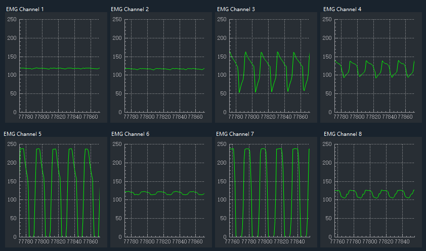
Figure 1. Eight channel EMG signal acquisition program

The sliding window method implements a window in time series data, and then moves this window slowly to perform the mean operation on the data within this window, and the result obtained is shown in Figure 2.

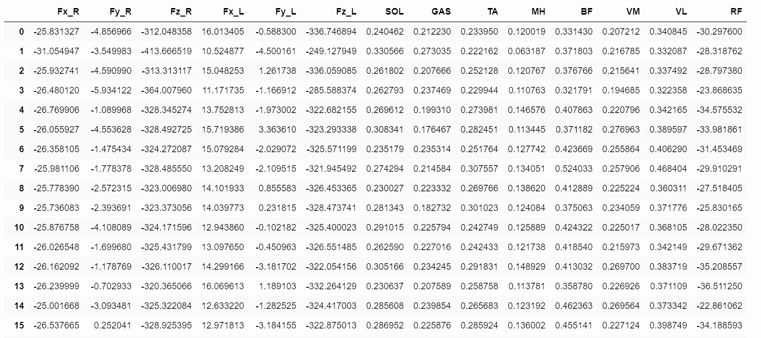
Figure 2. The result of EMG signal sliding window processing by Python

For neural networks and machine learning models, data normalisation can significantly accelerate the convergence of the model, and small-scale data are easier to learn. The formula for data normalisation is as follows:

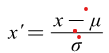
Where represents the mean of the input data and is the standard deviations of the input data. The distribution of normalized EMG characteristic is shown in Figure 3.

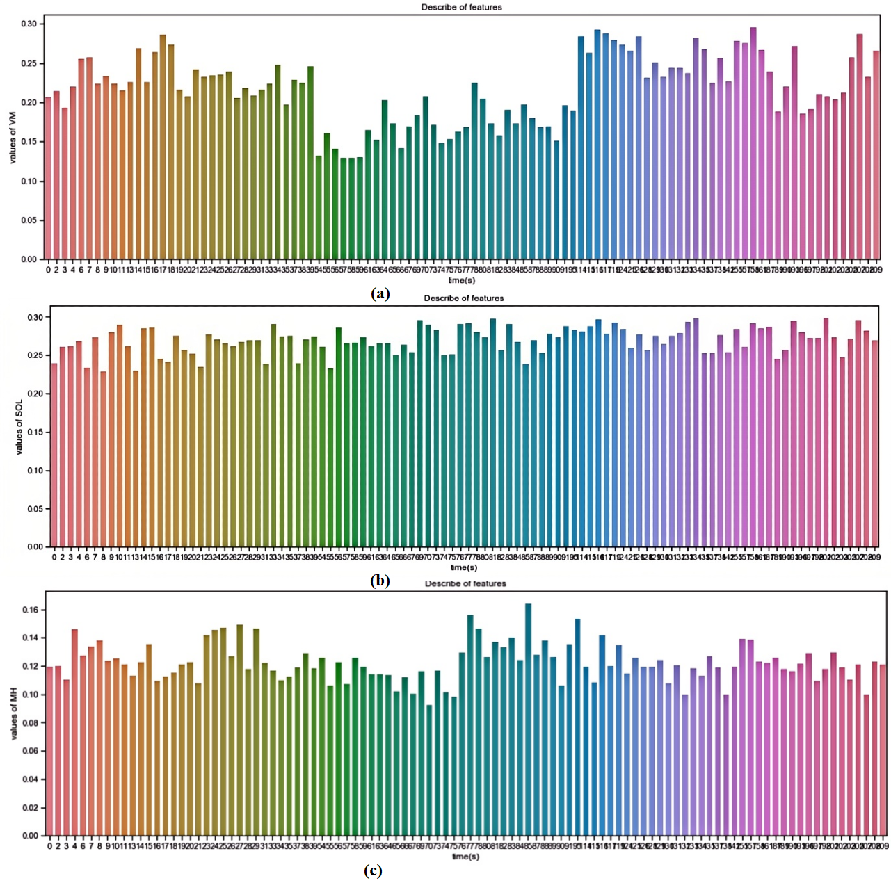
Figure 3. Distribution of normalized EMG characteristic Data (Y-axis represents value, X-axis represents time). (a) VM in medial thigh and thigh. (b) Sol in soleus. (c) MH in medial hamstring

2) Exploratory Data Analysis (EDA) and feature engineering: The first part is to filter and pre-process the input signal. In this paper, we complete the "data cleaning" by graphing, fitting, correlation analysis between features, observing and calculating the amount of features, correlation coefficients, etc.

Feature engineering is strictly a post-processing part of machine learning that analyzes the input and output data and the correlation between the input and output features to eliminate some obvious useless features, (Figure 4). Analyzing the correlation between the input features and true label values allows us to determine whether there is a significant positive correlation between the causality of all feature variables and the results in the dataset itself.

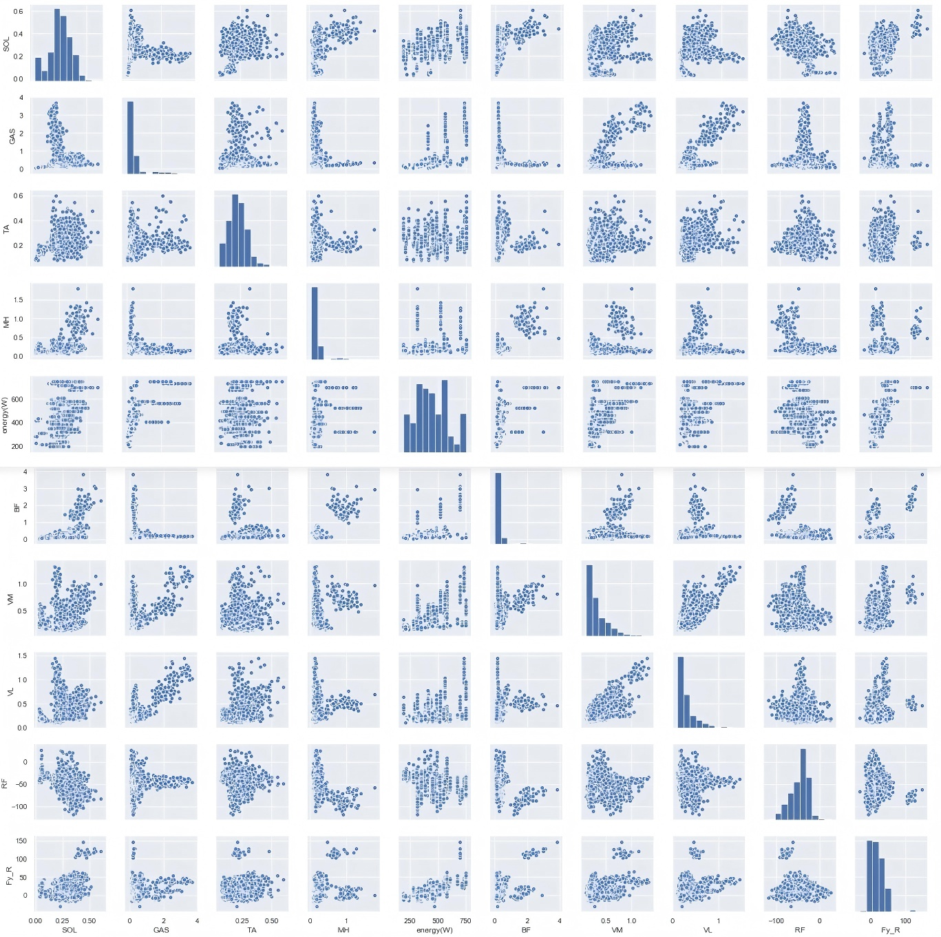
Figure 4. Correlation analysis chart between input features and between input and output

From the frequency histogram shown in Figure 5, we can determine whether the feature data are normally distributed, left-skewed, or right-skewed. Therefore, the data can be determined artificially to obtain an a priori understanding of the association between the data and EE.

Figure 5. Normalized Frequency histogram of EMG features...

3) Root Mean Square Error (RMSE) evaluation index: The output loss was used for the accuracy assessment. The loss function of the regression is the RMSE; the lower the RMSE, the more accurate the predicted value, which is given by the following formula:

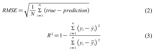
Where yi represents each observation point, the upper equation represents the distance between the regression curve (predicted value distribution curve) obtained from the model fit and the observation point, and the lower equation represents the mean value and distance between each observation point. The coefficient of determination is used to indicate how well the regression model is trained and is a regression model-specific metric.

B.  Machine learning regression-based modeling of EE

1) Decision tree-based modeling of EE: The boosting algorithm is the basis for the GBDT, and the objective of the GBDT is the residual, that is, the negative gradient value of the loss function.  Thus, boosting and decision-tree algorithms can help each other. XGBoost and GBDT are engineering implementations of the boosting algorithms.

This subsection focuses on the advanced part of XGBoost when compared to the GBDT from the perspective of the loss function and points out some advantages and disadvantages of the algorithm.

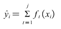
The essence of the boosting algorithm is a summation expression comprising j-base learners.

Where is the jth base learner, and  is the predicted value of the ith sample.

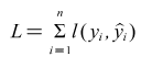
The loss function can be represented by the operations of the predicted and true values.

 

Where n is the total number of samples, and L is the loss function, such as the root mean square error operation RMSE or mean square error MSE.

Machine learning is a statistical learning method that measures the accuracy of a model in two ways: bias and variance of the model. The loss function represents the bias of the model; if the variance of the model is small, the model should be simpler.

The complexity of the model can be controlled by adding a regular term to its loss function. If the loss function minimises the empirical risk of the model, then the regularity term minimises its structural risk. Thus, the variance of the model is reduced, and the function composed of the regular term and the loss function becomes the objective function.

   

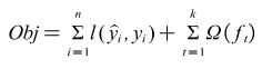
Where Ω is the regularization term of the model, the so-called regularization term is generally used L₁ regularization and L₂ regularization, and its formula is as follows.

 

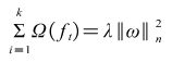
Where  is the parameterisation of weight . In , this term is the sum of the squares of the . In , this term is the sum of absolute values of .

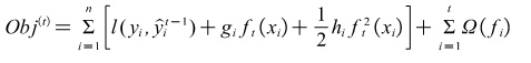
Specifically, the objective function of XGBoost can be written as the following equation.

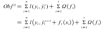
Where  is the predicted value given by the model at step (t-1), which is a known constant,  is the new model added at step t, and  is the predicted value of the newly added model. In other words, the optimisation of the objective function is equivalent to solving for the minimum value of .

In XGBoost, a second-order Taylor expansion is performed for , which is the main difference from the GBDT.

The second-order Taylor expansion is formulated as follows.

The expanded objective function equation is as follows.

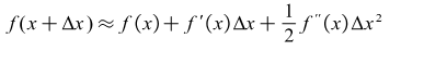
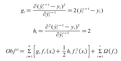
Where and  are the first-and second-order derivatives of the loss function, respectively.

If the loss function  is the squared loss function MSE, then  and  are as follows.

Minimising the objective function is transformed into determining the values of the first- and second-order derivatives of the loss function in each step.

The drawback of the XGBoost algorithm is that there is duplication in the reading of the dataset at each iteration, which slows the operation. Therefore, Lightgbm, a lightweight approach, was proposed that is similar to the mathematical principle of XGBoost.

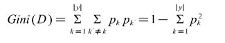
D is the set of data sets, the proportion of the kth category of samples in D is , and the Gini index reflects the probability of inconsistency between the categories of any two samples drawn from the data set D. The smaller the Gini value, the purer and more similar the information of the divided data set.

2) Time series data set partitioning and result evaluation methods: A time-series dataset is a one-dimensional feature graph of non-exchangeability. In a regression, it can only be iterated sequentially. This non-exchangeability of the time series has a significant impact on machine learning training.

Training set partitioning was required for both individual model training and subsequent model fusion training using k-fold cross-validation. In this study, k-fold cross-training was improved using a self-coding dataset partitioning n to reasonably partition the data according to the time series, which is called the improved k-fold cross-validation method. Two types of partitioning methods are used.

The first division is incremental and progressive, and the second division is similar to the idea of a sliding window. In this experiment, the second method was applied to improve the model fusion stacking algorithm, and the stacking dataset was improved from 5-fold cross-validation (chaotic order) to sliding window dataset division, which could effectively prevent the data from chaotic order and the training data from being clearly divided.

The experimental data were taken from the publicly available dataset in Slade's paper [20], as the dataset for model training and evaluation. The model evaluation results are shown in Table 1. In this experiment, the improved five-fold cross-validation method was used to predict one-dimensional time series data, and the results obtained are shown in Table 1.

Table 1.  Comparison of regression algorithm to estimate EE using 14 Signals (accuracy calculated by R2)

Regression model	Training set error	Training time (hours)	Test set error
GDBT Regressor	0.634	3.66306	0.980499
XGBoosting Regressor	0.999992	1.59833	0.977108
Lightgbm Regressor	0.994009	1.85351	0.975515
Bagging Regressor	0.993533	1.88308	0.971504
Lasso Regressor	0.987572	1.035499	0.950718
Ada Boost Regressor	0.95363	5.08391	0.940901
Decision Tree Regressor	1	1.317957	0.928449
Linear Regression	0.934234	1.34074	0.927853

The training set error is a measure of how well a model fits the dataset and the test set error is a measure of how well the model generalises. Precision is measured by the R² coefficient of determination, and the closer the coefficient is to 1, the better the curve fit.

As can be seen from Table 1, individual decision tree models have a tendency to overfit and are therefore discarded; however, CART decision tree-based models, such as the GBDT and XGBoost models, have a top level of both accuracy and speed for fitting such nonlinear relationships.

Table 2 lists the results of applying feature engineering to predict the human energy consumption. In Table 2, compared with Table 1, some features were excluded for retraining, and the input variables with a higher correlation in human energy consumption prediction were identified by feature engineering. Among the three decision-tree models with the highest accuracy, Lightgbm improved from 0.975 to 0.978, GBDT improved from 0.980 to 0.984, and of the coefficient of determination of XGBoost improved significantly from 0.977 to 0.983.

The advantage of removing useless features (input features with a Pearson's correlation coefficient below 0.3, feature importance) is that in the case of a small data sample size (less than 10000 rows), the risk of overfitting can be effectively reduced from the perspective of data structure, and fewer data and more features tend to make the model overfit. Feature engineering artificially dimensions the input of a dataset, thereby reducing the generalization error of the results.

Table 2.  Comparison of Regression Algorithm to Estimate EE using 8 Signals (accuracy calculated by R2)

Regression model	Training set error	Test set error	Test set standard deviation	Training time (hours)
GDBT Regressor	0.996631	0.984573	0.00677779	0.0821779
XGBoosting Regressor	0.999935	0.983237	0.00543861	0.172541
Lightgbm Regressor	0.996511	0.97815	0.0028755	0.0761986
Bagging Regressor	0.988732	0.9777757	0.00162806	0.160177
Lasso Regressor	0.890293	0.887219	0.01079	0.0141561
Ada Boost Regressor	0.911548	0.878368	0.0172662	0.229886
Decision Tree Regressor	1	0.867775	0.01079	0.0177521
Linear Regression	0.802545	0.772079	0.0550461	0.108515

As shown in Figures 6-8, it can be seen from Tables 1 and 2 that the decision-tree-based algorithms had the highest accuracy among all models. The decision tree-based algorithms XGBoost, GBDT, and Lightgbm have better generalisation performance for fitting nonlinear relationships, with a decision coefficient as high as 98.45%; however, in the test set data, The RMSE still has a deviation of approximately 30-70w and the prediction is high compared to the actual value.

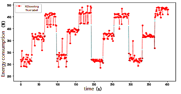
Figure 6. XGBoost time series diagram for predicting human energy consumption

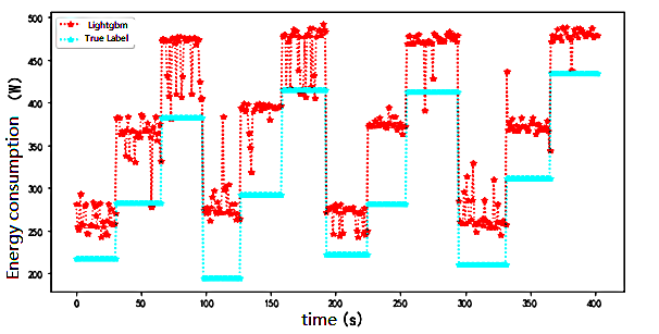
Figure 7. LightGBM time series diagram for predicting human energy consumption

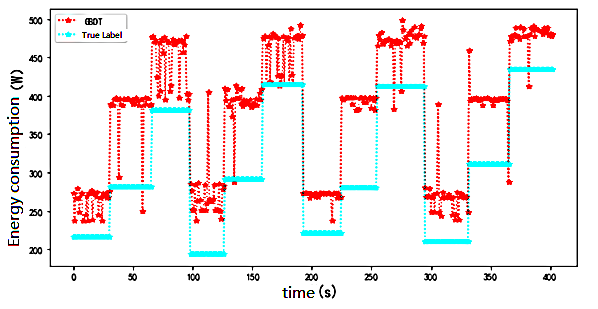
Figure 8. GBDT time series diagram for predicting human energy consumption

In the Lightgbm prediction , the lower deviation was approximately 30w and the higher deviation was 100w, which shows that the variance of the model prediction is larger. This explains the final RMSE of approximately 70w. This is because the dataset is small, and Lightgbm is suitable for prediction on larger datasets to reduce the degree of overfitting, whereas the RMSE of the GBDT model is 71w.

This implies that reducing the variance of the model prediction and increasing the stability of the model prediction will be the next tasks to be performed. A common method for further reducing variance in model prediction is model fusion. Lasso regression is a model based on linear regression with an L₁ regular term to prevent overfitting, and has the advantages of fast convergence and high accuracy.

The degree of feature importance (DoI) is measured by the correlation of a particular feature or signal with the EE, and can be calculated using the following Pearson correlation:

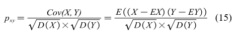
Where X is a feature; Y is the predicted EE; and EX and EY represent the mathematical expectations of X and Y, respectively. Here, as a post-processing, the predicted values according to the XGBoost model are taken in the experiment and the coefficients will vary between -1 and 1.  The definitions were as follows: very strong correlation (0.8, 1.0), strong correlation (0.6, 0.8), moderate correlation (0.4, 0.6), weak correlation (i.e., low DoI) (0.2, 0.4), and no correlation.

Figure 9 shows the importance of the 14 signals calculated using Equation (14). In Figure 9, the rows and columns represent different signals. The first column on the left side of Fig. 9 indicates the correlation between the different signals and the energy consumption.

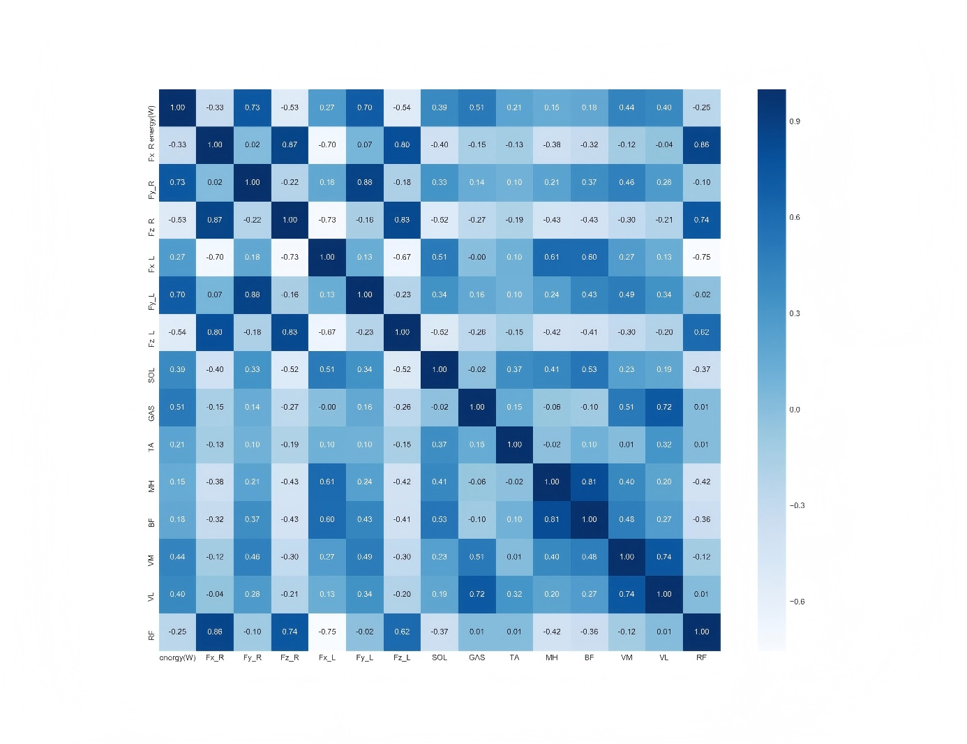
Figure 9. Calculated and sorted by Pearson correlation...

As shown in Figure 10, these six signals were the most important among the 15 signals. The EMG signals were those of the flounder, medial femoral, lateral femoral, and medial gastrocnemius muscles, and their human correlation coefficients were 0.39, 0.44, 0.40, and 0.51, respectively. In addition, the ground reaction force in the vertical direction showed a strong correlation with the EE owing to the tilt condition (Figure 11-15). Figure 15 shows the Pearson correlation coefficients of the six signals. From the analyses in Figure 14 and Figure 15, it can be observed that the EMG signals GAS,VM,VL, and SOL have a large influence on the predicted result Y_predict(energy(W)) of the XGBoost model among all features with a moderate correlation. Considering that there may be too much noise in this part of the data collection process, or that this part of the muscle itself has little influence on the prediction results, this part of the dataset may have a negative impact on the results. These three features were randomly removed, redundant ground reaction force features were removed, and only the six variables shown in the figure below were retained as input features. The results are summarised in Table 2. The accuracy and model training speed were further improved compared to those in Table 1.

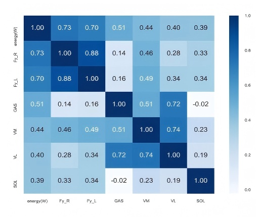
Figure 10. The six most important features based on the Pearson coefficient

C.  Fused models

The specific processes of XGBoost and Lightgbm fusion in this experiment are shown in Figure 11. However, the stacking algorithm has the drawback that it is disordered when it performs dataset partitioning, which is contrary to the strict temporal characteristics of the time-series problem. In this study, the dataset partitioning strictly followed the concept of temporal order to obtain an improved stacking algorithm.

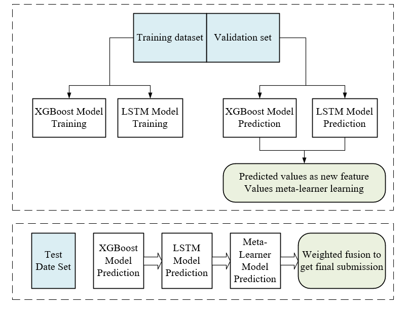
Figure 11. Training diagram of stacking algorithm

The training diagram of the improved stacking algorithm is shown in Figure 12. The subsequent time steps were followed in this way: 20% of the data were taken as the training set and 20% of the data were taken as the validation set, until the data were taken, and the prediction results of the five steps were finally averaged as the final output.

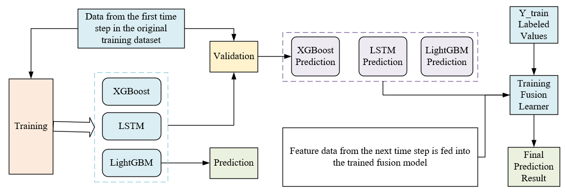
Figure 12. Training diagram of improved stacking algorithm

Results and discussion

A.  Model fusion based on XGBoost, GBDT and Lightgbm

As shown in Figure 13, the dataset and features used were consistent with the experiments used in Table 2. The RMSE of this model fusion in the prediction results of the test set was reduced from about 66-70 W for the original single model to 51 W, which significantly improved the accuracy of the model. From the entire timestamp, the results of model fusion are closer to the real label than those of the single model. Thus, the real label values of human energy consumption can be better fitted. The best prediction results were obtained in the time steps of 0s–25s, 200s to 250s and 300–325s, but there were still some prediction results with a large offset from the true value.

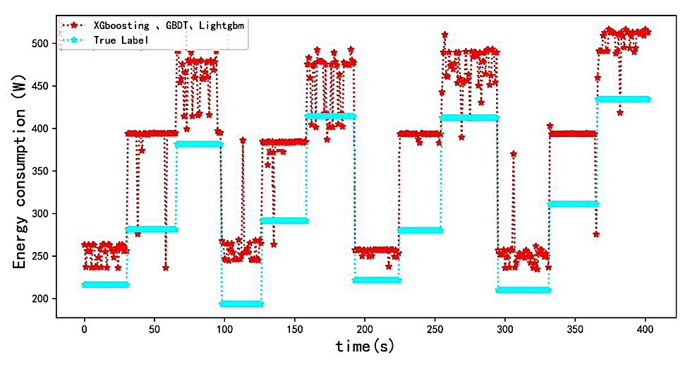
Figure 13. Comparison of stacking prediction results with real Tags

Both XGBoost and Lightgbm are nonlinear models based on Cart decision regression trees, and the accuracy adjustment of the models plays a crucial role in whether the models can achieve the highest accuracy. The correlation analysis of primary learners in Stacking is shown in Figure 14. The following provides a further description of the XGBoost model parameters and their mathematical principles. One of the most important hyperparameters is learning_rate, which is set to 1 by default and is also the weight reduction factor of each weak learner, also called the step size. The subsample is the sampling ratio of the training samples, that is, the subsampling of the dataset, and takes the value (0,1). Here, 0.8 is chosen as the result.

Figure 14. Correlation analysis of primary learners in stacking

N_estimators indicate the number of boosted trees, that is, the number of training rounds, and the 1500 effect was measured in the experiment. By writing the model parameter search function, the loss of model training was reduced to a minimum when the learning rate was 0.0004887 and n_estimators=300 in the model selection parameters were obtained. The remaining parameter combinations are obtained by manual tuning of the parameters according to experience, and the global optimum is obtained (Figure 15).

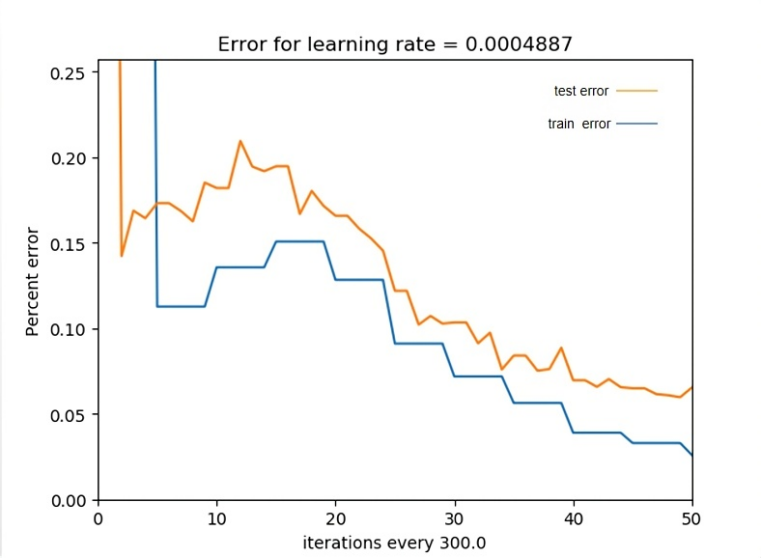
Figure 15. Visualization of stacking training process — percentage error reduction

The blue and yellow lines represent the training and test set losses, respectively. By adjusting the learning rate of the model parameters n_estimators, the test set error is made as close as possible to the training set error so that the results converge.

B.LSTM based energy consumption expenditure prediction

1) Analysis of LSTM principle: LSTM is a recurrent neural network that recirculates the output as an input for the next time step for each neuron. It has the advantage of being able to influence subsequent events by the previous moment's events, that is, a memory function. However, recurrent neural networks can have a problem in that there is less influence on the initial time-step weights because of the gradual derivation of the error during backpropagation. LSTM improves the easy-forgetting properties of traditional recurrent neural networks by introducing a three-class gate structure.

As shown in Figure 16, the LSTM contains three main types of gates internally, and the three types of gate structures have three functions, i.e., forgetting gate, input gate, and output gate.

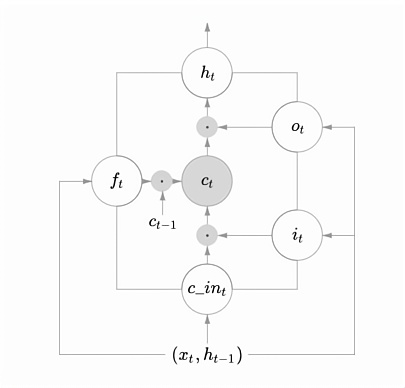
Figure 16. LSTM internal gate logic diagram

The forgetting gate equation is shown in (16).

 

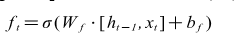
Where is the output of the previous moment, is the current input, the obtained  is a value in the range of 0-1. The primary role of the forgetting gate is to actively control the forgetting process.

The input gate formula is shown in (17).

 

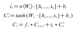
The input gate contains three parts, the first part is used to decide which parts should be taken to memory for this input by the sigmoid function. The second part is used to generate a new state variable  for the next layer of the forgetting gate update. In the third part, the previous state variable  is forgotten by the forgetting gate, and the state variable  at the current moment is selectively learned, and the weighted sum is obtained for the real learned variable  at the current moment.

The output gate equation is shown in (18).

 

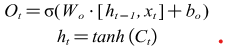
Among the output gates, the standard output  is obtained by calculating the output  learned from the input data at the current moment and the cumulative knowledge  learned at the previous moment, weighted and then compressed to the range of -1~1 by the tanh function.

From Figure 17, it can be seen that the single LSTM model has a good fit for human energy consumption prediction, whereas in the case of consistently high prediction based on the decision tree model, the LSTM model regressed above and below the true value.

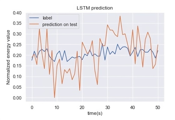
Figure 17. Comparison of prediction results and real values based on LSTM model

However, variance and bias values were high. The accuracy measure RMSE was 127.778 W, which was significantly higher than those of the XGBoost, GBDT, and Lightgbm models.

However, from the perspective of model fusion, the fusion of LSTM with XGBoost and Lightgbm may compensate for high prediction results. It is known from the previous experiment that model fusion can significantly reduce the variance of the prediction results. Although the variance of the results is reduced, the problem of high prediction results still remains.

In LSTM, XGBoost, and Lightgbm for model fusion, we tried to maintain the same dataset selection and model hyperparameter selection as in the previous experiment and only changed the GBDT in the primary learner to LSTM for cross-sectional comparison using this method.

As shown in Figure 18, one disadvantage of the LSTM is that the number of training iterations is significantly higher than that of the decision-tree-based model.

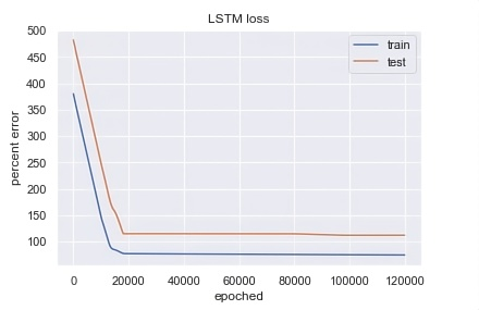
Figure 18. Percentage error of training set and prediction set in LSTM training

2) LSTM parameter setting and experimental procedure: The LSTM model is built in general with the following parts.

In the first step, the dataset is loaded and normalized.

The second step is to slide the dataset in a time window using the shift function inside the pandas and then splice it into the original dataset after it becomes new data.  

The third step is to slice the dataset and cut the dataset in order, taking 20% as the training set and 20% as the validation set. Subsequently, the algorithm iterates sequentially until the entire dataset is traversed.

The fourth step is to convert the training and validation set data into the input data format of the LSTM.

The fifth step is to design the network structure, which is the most important part of the LSTM model setup. The LSTM model is a stitching of each LSTM cell mentioned in the previous subsection; therefore, setting up the LSTM cells is the first step in the model design. Subsequently, the dense structure, which is the same as the structure of each layer of an ordinary ANN, was used for the regression prediction. In addition, a loss function optimiser for the model must be set up. Networks differ from traditional regression algorithms like decision trees in that they use a back propagation algorithm to reduce the loss, where the 'Adam' optimiser is often used for its fast convergence and high accuracy. The loss function was set to the RMSE.

In the sixth step, the parameters are set and tuned. The main parameters were the epoch (number of iterations) of the model, batchsize, and input batch. This part was manually tuned to determine whether the training was overfitting, by observing whether the loss of the validation set was reasonably low.

As shown in the comparison between Figure 19 and Figure 9, the correlation between the output energy and each input feature is significantly different between the two plots, and the importance of the features and the correlation between the features learned by the LSTM are completely different from those learned by the decision-tree-based model.

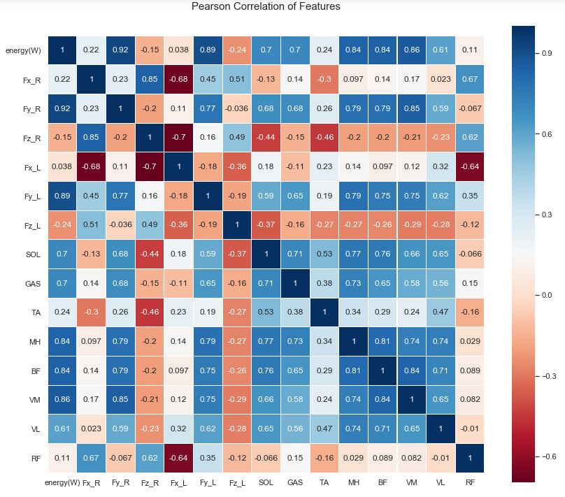
Figure 19. Visualization of LSTM training process percentage error

For the LSTM model, VL, VM, BF, and MH are strongly correlated variables; therefore, these features cannot be eliminated and are important for the prediction results, which is again very different from the conclusions obtained in previous feature engineering using XGBoost. From this, we can observe that the mapping relationship between the input and output learned by the LSTM is completely different from that of the previous XGBoost model. The focus of the LSTM model and XGBoost are different, and LSTM gives more weight to VL, VM, BF, and MH; therefore, these two different models can complement each other when fused to further reduce variance and enhance generalisation.

C.Model fusion based on XGBoosting, LSTM and Lightgbm

The purpose of this experiment was to analyse and investigate the best combination of model combinations for model fusion. For the fitting of nonlinear relationships, the effects of traditional linear regression and Lasso regression based on linear regression as the base learner were not satisfactory. The LSTM neural network, as a completely different algorithm from the decision tree algorithm, can also be concluded from the previous subsection to have a better prediction ability for this type of nonlinear problem. Therefore, an attempt was made to fuse the decision-tree and LSTM algorithms to determine the best model combination.

From Figure 20, it can be seen that the model fusion algorithm based on XGBoost and LSTM can effectively reduce the RMSE of the model, which is lower than the RMSE value of the XGBoost, GBDT, and Lightgbm model fusion. An RMSE of 25 W enabled the overall prediction to reach a very high level of accuracy. Unlike the high results obtained by the decision-tree-based model fusion, the LSTM algorithm effectively compensates for the problems of the decision-tree-based XGBoost and Lightgbm algorithms, as the results are regressed above and below the true values.

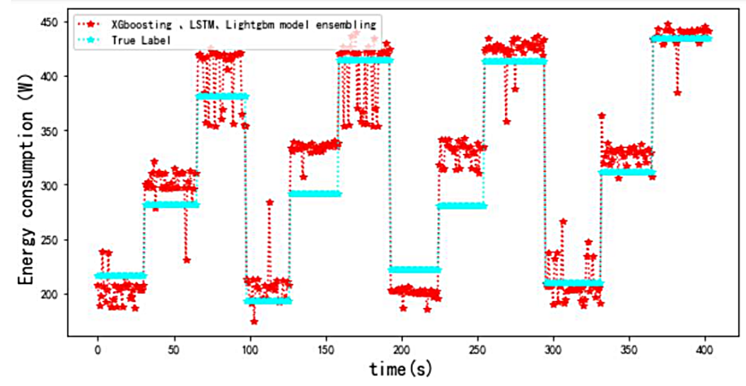
Figure 20. Comparison of stacking prediction results with real Tags

In Figure 21, the yellow line represents the validation set error, and the blue line represents the prediction set error. If the number of iterations increases, the training set error decreases and the validation set error increases, indicating that the model overfits and can be improved by feature engineering or by adding regular terms.

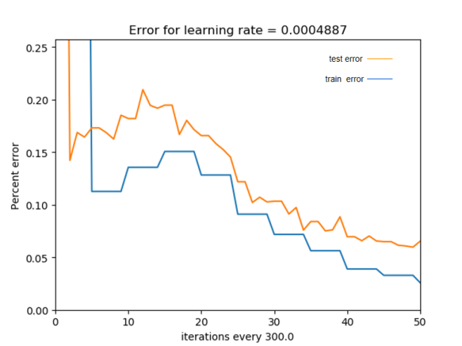
Figure 21. LightGBM training process — percentage error reduction

If the training set error decreases and the validation set error decreases, there is still a gap between the two, indicating that the loss function of the model does not decrease and the prediction ability of the model for the problem reaches the upper limit, which can only be solved by replacing the model or the dataset. If the error of the training set is elevated, it indicates that there is a problem with the dataset, and data cleaning is required to exclude anomalies. The final stacking model was obtained by fusing the LSTM, XGBoost, and Lightgbm algorithms. The model selection and construction of a human energy consumption prediction system that can be applied to practical predictions were obtained by introducing LSTM models with significant improvements in accuracy and generalisation performance at the expense of computing speed.

A comparison of the stacking model prediction timing diagram and real labels suggests that the stacking algorithm is more accurate and stable than the individual models. In addition to the comparison between Figure 22 and Figure 14, it can be concluded that the fusion of models based on different principles offers better accuracy in estimating the EE, and the model generalisation performance was significantly improved.

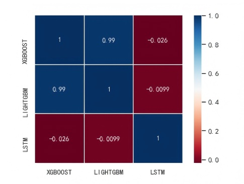
Figure 22. Model correlation calculation based on Pearson coefficient

The prediction results of the decision tree models are very similar; therefore, their model fusion can only reduce the impact of individual outliers on the overall model and cannot solve the overestimation issue, which is a common problem in decision tree model prediction. Unlike LSTM, the distribution of the prediction results was completely different from that of XGBoost and Lightgbm. The correlation is very low, and the individual prediction values are lower than the true values. Thus, the fusion of the two different types of models can effectively reduce the overestimation rate.

Conclusion

EE is widely applied in sports, rehabilitation loss and exoskeleton design, but traditional measurement methods are time-consuming and laborious, therefore, fast and accurate sensor-based algorithms has become a top priority in this field. In this study, surface EMG sensors and machine learning algorithms were used for the prediction of EE. For nonlinear problems such as EE prediction, the Pearson correlation coefficient analysis between the input features was first proposed, the fitting coefficient of the XGBoost model before and after the feature engineering increased from 0.977 to 0.983. The machine learning fusion algorithm of time series prediction was improved and optimized, and the improved stacking algorithm was proposed. The model fusion by XGBoost and Lightgbm reduces the RMSE from 60-70W in a single model to 51W. It demonstrated that the improved model can reduce the prediction error and improve the stability. The model fusion algorithm of LSTM, XGBoost and Lightgbm gave a higher accuracy for EE prediction, and the RMSE is reduced from 51W to 25W again, with an improvement of accuracy of nearly 64%, and the timing diagrams are also more stable.

Conflicts of interest

The authors declare that they have no conflict of interest.

Acknowledgement

This work was financially supported by the National Administration of Traditional Chinese Medicine Scientific Research Project-System Construction, Evaluation and Application of Pingle Bone Setting for Prevention and Treatment of Knee Osteoarthritis (GZK-KJS-2023-012).

References

1. Hamilton MT, Hamilton DG, Zderic TW (2007) Role of low energy expenditure and sitting in obesity, metabolic syndrome, type 2 diabetes, and cardiovascular disease. Diabetes 56: 2655-2667. [Crossref]
2. Nordstoga AL, Zotcheva E, Svedahl ER, Nilsen TIL, Skarpsno ES (2019) Long-term changes in body weight and physical activity in relation to all-cause and cardiovascular mortality: The HUNT study. Int J Behav Nutr Phys Act 16: 45. [Crossref]
3. Margaria R, Cerretelli P, Diprampero PE, Massari C, Torelli G (1963) Kinetics and mechanism of oxygen debt contraction in man. J Appl Physiol 18: 371-377. [Crossref]
4. Chang Y, Kang J, Jeong B, Kim G, Lim B, et al. (2023) Verification of industrial worker walking efficiency with wearable hip exoskeleton. Appl Sci 13: 12609. [Crossref]
5. Ekegren CL, Beck B, Climie RE, Owen N, Dunstan DW, et al. (2018) Physical activity and sedentary behavior subsequent to serious orthopedic injury: A systematic review. Arch Phys Med Rehabil 99: 164.e6-177.e6. [Crossref]
6. Lipperts M, van Laarhoven S, Senden R, Heyligers I, Grimm B (2017) Clinical validation of a body-fixed 3D accelerometer and algorithm for activity monitoring in orthopaedic patients. J Orthop Translat 11: 19-29. [Crossref]
7. Compagnat M, Mandigout S, Batcho CS, Vuillerme N, Salle JY, et al. (2020) Validity of wearable actimeter computation of total energy expenditure during walking in post-stroke individuals. Ann Phys Rehabil Med 63: 209-215. [Crossref]
8. Bamberga M, Rizzi M, Gadaleta F, Grechi A, Baiardini R, et al. (2015) Relationship between energy expenditure, physical activity and weight loss during CPAP treatment in obese OSA subjects. Respir Med 109: 540-545. [Crossref]
9. Mitchell L, Wilson L, Duthie G, Pumpa K, Weakley J, et al. (2024) Methods to assess energy expenditure of resistance exercise: A systematic scoping review. Sports Med 54: 2357-2372. [Crossref]
10. Udomtaku K, Konharn K (2020) Energy expenditure and movement activity analysis of sepaktakraw players in the Thailand league. J Exerc Sci Fit 18: 136-141. [Crossref]
11. Fang Z, Chen L, Moser MAJ, Zhang W, Qin Z, et al. (2021) Electroporation-based therapy for brain tumors: A review. J Biomech Eng 143: 100802. [Crossref]
12. Wang F, Qian Z, Lin Y, Zhang W (2021) Design and rapid construction of a cost-effective virtual haptic device. IEEE/ASME Transactions on Mechatronics 26: 66-77.
13. Yin R, Qian X, Kang L, Wang K, Zhang H, et al. (2021) A step towards glucose control with a novel nanomagnetic-insulin for diabetes care. Int J Pharm 601: 120587. [Crossref]
14. Modi S, Tiwari MK, Lin Y, Zhang WJ (2011) On the architecture of a human-centered CAD agent system. Comput Aided Des 43: 170-179.
15. Schoeller DA (1988) Measurement of energy expenditure in free-living humans by using doubly labeled water. J Nutr 118: 1278-1289. [Crossref]
16. Schoeller DA, Luke AH (1997) Rapid 18O analysis of CO₂ samples by continuous-flow isotope ratio mass spectrometry. J Mass Spectrom 32: 1332-1336. [Crossref]
17. Wu ZF, Li J, Cai MY, Lin Y, Zhang WJ (2016) On membership of black-box or white-box of artificial neural network models. In 2016 IEEE 11th Conference on Industrial Electronics and Applications (ICIEA) 1400-1404.
18. Modi S, Lin Y, Cheng L, Yang G, Liu L, et al. (2011) A socially inspired framework for human state inference using expert opinion integration. IEEE/ASME Transactions on Mechatronics 16: 874-878.
19. Ravussin E, Harper IT, Rising R, Bogardus C (1991) Energy expenditure by doubly labeled water: Validation in lean and obese subjects. Am J Physiol 261: E402–E409. [Crossref]
20. Migueles JH, Cadenas-Sanchez C, Ekelund U, Delisle Nyström C, Mora-Gonzalez J, et al. (2017) Accelerometer data collection and processing criteria to assess physical activity and other outcomes: A systematic review and practical considerations. Sports Med 47: 1821-1845. [Crossref]
21. Slade P, Troutman R, Kochenderfer MJ, Collins SH, Delp SL (2019) Rapid energy expenditure estimation for ankle assisted and inclined loaded walking. J Neuroeng Rehabil 16: 67. [Crossref]
22. Weir J B de V (1949) New methods for calculating metabolic rate with special reference to protein metabolism. J Physiol 109: 1-9.
23. Cvetković B, Milić R, Luštrek M (2016) Estimating energy expenditure with multiple models using different wearable sensors. IEEE J Biomed Health Inform 20: 1081-1087. [Crossref]
24. Rosic G, Pantovic S, Niciforovic J, Colovic V, Rankovic V, et al. (2011) Mathematical analysis of the heart rate performance curve during incremental exercise testing. Acta Physiol Hung 98: 59-70. [Crossref]
25. Schmitz KH, Treuth M, Hannan P, Mcmurray R, Ring KB, et al. (2005) Predicting energy expenditure from accelerometry counts in adolescent girls. Med Sci Sports Exerc 37: 155-161. [Crossref]
26. Ainsworth BE (2000) Compendium of physical activities: An update of activity codes and MET intensities. Med Sci Sports Exerc 32: S498.
27. Dal U, Erdogan T, Resitoglu B, Beydagi H (2010) Determination of preferred walking speed on treadmill may lead to high oxygen cost on treadmill walking. Gait Posture 31: 366-369. [Crossref]
28. Ryu N, Kawahawa Y, Asami T (2008) A calorie count application for a mobile phone based on METS value. In 2008 5th Annual IEEE communications society conference on sensor, mesh and ad hoc communications and networks 583-584.
29. Katch V, Becque M, Marks C, Moorehead C, Rocchini A (1988) Oxygen uptake and energy output during walking of obese male and female adolescents. Am J Clin Nutr 47: 26-32. [Crossref]
30. Hibbing PR, Lamunion SR, Kaplan AS, Crouter SE (2018) Estimating energy expenditure with actigraph GT9X inertial measurement unit. Med Sci Sports Exerc 50: 1093-1102. [Crossref]
31. Tikkanen O, Kärkkäinen S, Haakana P, Kallinen M, Pullinen T, et al. (2014) EMG, heart rate, and accelerometer as estimators of energy expenditure in locomotion. Med Sci Sports Exerc 46: 1831-1839. [Crossref]
32. Hedegaard M, Anvari-Moghaddam A, Jensen BK, Jensen CB, Pedersen MK, et al. (2020) Prediction of energy expenditure during activities of daily living by a wearable set of inertial sensors. Med Eng Phys 75: 13-22. [Crossref]
33. Altini M, Casale P, Penders J, Amft O (2015) Personalized cardiorespiratory fitness and energy expenditure estimation using hierarchical Bayesian models. J Biomed Inform 56: 195-204. [Crossref]
34. Lin CW, Yang YT, Wang JS, Yang YC (2012) A wearable sensor module with a neural-network-based activity classification algorithm for daily energy expenditure estimation. IEEE Trans Inf Technol Biomed 16: 991-998. [Crossref]
35. Catal C, Akbulut A (2018) Automatic energy expenditure measurement for health science. Comput Methods Programs Biomed 157: 31-37. [Crossref]
36. Nathan D, Huynh DQ, Rubenson J, Rosenberg M (2015) Estimating physical activity energy expenditure with the kinect sensor in an exergaming environment. PLoS One 10: e0127113. [Crossref]
37. Khan AM, Lee YK, Lee SY, Kim TS (2010) A triaxial accelerometer-based physical-activity recognition via augmented-signal features and a hierarchical recognizer. IEEE Trans Inf Technol Biomed 14: 1166-1172. [Crossref]