Predicting the onset of a manic episode so that timely medical intervention can occur is an important issue in the long-term management of people diagnosed with Bipolar I Disorder. In this proof-of-concept investigation of a single case, activity time series acquired from a wrist-worn actigraph were used to detect quantitative precursors of a manic episode that resulted in the hospitalization of a young man diagnosed with the disorder at the end of week 14. Using transformed activity data, a multifractal analysis showed that the data were significantly multifractal as indicated by the lack of overlap between Hurst functions computed from the data and surrogate series. When a continuous Shannon entropy measure derived from a lognormal distribution was fit to the multifractal spectra for each of the 14 weeks of data, a decrease in entropy of practical significance was observed after week 12. If this newly discovered indicator of relapse had been used to initiate preventative treatment, it is possible that hospitalisation might have been avoided. As this analysis is based on a single case study and just one episode, larger samples will need to be prospectively monitored into manic and depressive relapses to generalize the proposed methodology and permit its widespread usage for automated episode monitoring and prevention.
actigraphy, entropy, mania, multifractal, relapse
Bipolar disorder, a severe psychiatric condition with a lifetime prevalence of about 2% [1] is characterised by episodes of severe depression and mania interspersed with euthymic periods during which the patient is relatively well. Bipolar disorder generates significant morbidity and mortality, and is a significant financial burden for health care systems. Although the burden from bipolar depression can be extremely debilitating, manic episodes are the most functionally impairing phase of the disorder, frequently accompanied by psychosis, hyperactivity and sleep disturbance, leading to protective hospitalisation [2]. By identifying manic episodes early, less aggressive interventions, such as stimulation reduction and an increase in antipsychotic medication, may lead to euthymia.
Bipolar patients who respond swiftly to early indicators of an episode have better outcomes [3]. As commonly-used daily mood monitoring is not ideal because of patient burden and impaired insight, 24-hour activity monitoring can provide automated, objective information about episode prodromes [4].
Fluctuations in activity during any 24-hr period provide information about the variability of the associated psychomotor process. As in any time series, variability can be random or regular, the extent of this randomness being reflected in complexity measures such as the correlation dimension for series that have nonlinear or perhaps chaotic properties [5]. Research in a number of biomedical domains has found that a significant decrease in complexity may indicate the onset of pathology [6]. For example, chronic disorders are characterized by reduced complexity in measures such as heart-rate for heart disease, EEG amplitude and frequency for epileptic seizures, and mood rating variability for people with depression [6]. Perhaps a loss of complexity might be associated with the imminent onset of a manic episode.
This study interrogated multi-day actigraphy data to determine whether complex nonlinear dynamic analyses could predict transition from euthymia to mania using unique prospective data obtained as a patient progressed from euthymia into a full-blown manic episode.
A characteristic feature of mood disorder is the observed fluctuations in activity levels exhibited by patients as their mood changes. One of the early signs of depression, for example, is a reduction in activity level as the patient withdraws from their usual activities and leads a more sedentary life. On the other hand, incipient mania typically appears as increased physical activity and decreased sleep [7]. Indeed, changes in goal-directed activity are now recognised alongside mood changes as core diagnostic criteria for mania [8].
Human activity is commonly used to measure sleep and circadian rhythms under naturalistic conditions. The wrist-worn Actiwatch (Mini-Mitter Co., OR, USA) used in this project records three-dimensional movement using an accelerometer and on-board memory storage [9].
The raw actigraphy data analysed here have been described in a case report that used activity measurements collected by a wrist-worn actigraph to monitor the behavior of a 20-year-old male participant diagnosed with bipolar disorder Type I [4]. In this study, a plot of the raw actigraph data obtained two weeks prior to hospital admission showed that there was reasonably normal activity and sleep patterns for the first eight days followed by the sudden appearance of severely disrupted sleep and an increase in activity in the five days prior to hospitalisation. The sleep pattern changed to a 48-hour cycle and average activity levels increased markedly. We might expect, therefore, that a more detailed analysis of activity dynamics would reveal evidence of a decline in health at least a week before the hospitalisation occurred, if not earlier.
The participant was enrolled in a 12 month prospective study of actigraphically-measured sleep and circadian function as predictors of daily mood in bipolar disorder. For this patient, activity was recorded for 103 days prior to withdrawal from the study due to hospitalisation for a manic episode. The actigraph was removed on the first morning of admission to hospital as part of the routine procedure prior to commencement of treatment. Permission to conduct the study was obtained from the Swinburne University of Technology Research Ethics Committee and the patient provided written informed consent to take part in the study.
Data preparation
In the present paper, the data were analysed each week over 14 weeks starting at Day 5 to ensure that the final few days of recordings were included. The raw activity data were recorded every two minutes. For all analyses, the data were summed over five successive values so that activity recorded during each ten-minute period could be analysed. Pooling the data reduced the autocorrelation observed for successive two-minute observations. Due to large fluctuations in these pooled activity measures, each value was incremented by 1 and the logarithm was computed. Finally, the data were differenced to measure the change in log (activity+1) from one ten-minute time period to the next. This strategy removed any linear trend that might be present in the data.
Analysis of the activity data progressed in three stages. First, the power spectra were investigated using log-log transformations of both power and frequency. Detrended Fluctuation Analysis (DFA) was then used to test for long-range correlation. Finally multifractal spectra were explored to generalise the findings of the DFA and to calculate an appropriately sensitive index to indicate manic relapse.
Log-log power spectrum
As it has been shown [10], the power spectrum relating power to frequency for a time series such as activity can provide useful information about temporal dependencies in the series. In particular, when logarithms are taken of both the power and the frequency, the linearity of the log-log function has been associated with long-range correlations provided confirming evidence is obtained by applying other techniques such as Detrended Fluctuation Analysis (DFA).
Detrended fluctuation analysis (DFA) and the Hurst exponent
DFA has been used to quantify the fractal nature of a time series. A fractal is a mathematical object that is scale-invariant [11], so that no matter what time scale we choose to measure it, a fractal object always appears the same. In this case we assume that the activity time series, A(t), is time-scale invariant and satisfies the equation,  , where c is a scale constant and H is the Hurst exponent, a constant in this monofractal case. This self-similarity property, which occurs in many physiological time series such as heart rate, has also been found in actigraphy data during normal activity [12] and during sleep [13].
Before applying DFA, the mean activity is subtracted from each activity value. These differences are accumulated and the resulting function is fit by a linear relationship resulting in prediction errors. The mean fluctuation is obtained by taking the square root of the mean squared prediction error. This calculation is performed for nonoverlapping data intervals that increase in length from about 10 up to half the length of the time series. The slope of the linear relationship between the logarithm of the mean fluctuation and the logarithm of the interval length provides an estimate of monofractality known as the Hurst exponent, a number between 0 and 1. Knowing the Hurst exponent is useful because any value less than 0.5 indicates an antipersistent process that corrects itself if the values become too small or too large, whereas a Hurst exponent greater than 0.5 indicates a persistent process that tends to maintain its current state. Gaussian noise is characterized by a Hurst exponent equal to 0.5. As these processes can be represented by a single Hurst exponent, they are monofractal.
Multifractal spectral analysis of activity data
A multifractal process is a generalization of DFA to include processes for which the Hurst exponent is no longer constant over all time scales. Such processes are immensely complex. Examples from the physical world include atmospheric turbulence and water flowing over a waterfall. Evidence for a multifractal process is obtained when the Hurst exponent is not constant but depends on the fluctuation order, or fractal index [14].
Multifractal data analyses were conducted using Multifractal Detrended Fluctuation Analysis (MFDFA) [15,16] programmed in R (R 3.1.2 64-bit for Windows) [17]. The calculations used several data window sizes ranging from 23 = 8 to the power of two that is no greater than 20% of the number of observations in the time series. For activity accumulated over 10 min periods (1008 observations per week), the maximum window size is the largest integer less than log2(1008/5) = 7.7, which equals 7. The program returns the fluctuation function variance, the generalized Hurst exponent, the multifractal exponent, and the abscissa and ordinate of the multifractal spectrum (see [16] for technical details of this methodology). Cubic detrending, as used in these analyses, effectively controlled for nonlinear temporal variations, or nonstationarity, in the parameters responsible for variability in activity, as has been recommended in [18]. In the following analyses, the results were almost precisely the same irrespective of whether linear, quadratic or cubic detrending was applied.
As shown in [16], complex fluctuations in time series of various amplitudes can be evaluated by estimating the generalized Hurst exponent, Hq, for various values of, the fractal or singularity index, −5 ≤ q ≤ 5. If Hq does not depend on, the time series is monofractal implying that all types of fluctuations, large and small, scale in the same way. If Hq decreases as q increases, the time series contains fluctuations occurring on many different time scales leading to multifractality. Positive values of q reflect the effect of large-scale fluctuations, whereas negative values of q result from fluctuations with small variance.
The Hurst exponent computed by DFA is the value of Hq when q = 2, a special case of a monofractal. In the following analyses we will concentrate on the multifractal spectrum as computing a separate DFA analysis is redundant when a multifractal analysis is applied to data. The algorithm devised in [16], upon which this analysis is based, incorporates modifications recommended in [15] to accommodate instabilities that arise when q is close to 0 or negative.
The multifractal spectrum relates the multifractal amplitude, f (α), to the fractal index, α. For a sample from a normal distribution or monofractal series, the multifractal spectrum has a single value of 1 located at a value of α that corresponds to the DFA value, being 0.5 for the normal distribution and some other number between 0 and 1 for a monofractal series. This value will be equal to the Hurst exponent estimated using MFDFA when q = 2.
By contrast, the multifractal spectrum for the multifractal series is inverse parabolic in shape with a maximum value of 1 occurring for α lying between 0 and 1. As the width of the multifractal spectrum can be defined for any value of f (α), it is common to fit the spectrum with a quadratic polynomial, and identify the spectrum width with the distance between the roots of this best-fitting quadratic when f (α) = 0 [19].
Representation of a multifractal in terms of a Gaussian multiplicative Cascade
A common representation of a multifractal process is in terms of a multiplicative cascade as illustrated in Figure 1 [14]. The cascade operates on increasingly more precise time scales starting by dividing the full temporal interval by two at time scale T1 and continuing this division by two at each successive time scale, T2, T3, …,Tk. The flow of information from one time scale to the next is determined by the same probability density function, p(x). Eventually it is proposed that the cascade can produce the type of activity represented by that exhibited during Week 14 by the patient, as shown at the bottom of Figure 1.
Figure 1. A multiplicative cascade process driven by a general pdf, p(x), at increasingly fine binary time scales starting with the complete time interval at T0 and increasing the number of intervals by an integer power of two so that at time scale Tk the number of intervals is 2k. It is assumed that the activity time series shown at the bottom of the graph is generated by a multiplicative cascade in which p(x) is a Gaussian density with mean µ and variance σ2.
The challenge is to determine p(x) based on the form of the multifractal spectrum. For simplicity, we will assume that p(x) is the Gaussian probability density function (pdf) with mean, µ, and variance, σ2:
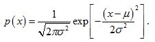 .
.
It can be shown [20] that the multifractal spectrum for a multiplicative cascade driven by a Gaussian pdf is given by
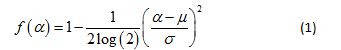
This theoretical multifractal spectrum attains its maximum value of 1 when α = µ and its width at f (α) = 0 is given by 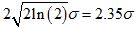 [19]. This means that in principle at least, estimates of the mean and variance of the presumed Gaussian pdf can be estimated by mere inspection of the empirical multifractal spectrum. Fitting Equation 1 to the multifractal spectrum obviates the need to estimate its peak location and width, two commonly used quantifiers of an empirical multifractal spectrum. This strategy renders superfluous a quadratic fit to the spectrum with its associated extrapolation uncertainty. Moreover, it provides a strikingly simple test of the Gaussian multiplicative cascade process, with its implications for a novel theoretical investigation of the temporal precursors of human activity generation.
The probability associated with each branch of a multiplicative cascade process can be constructed by applying a log transform to the product of random variables that are associated with that branch [20]. This results in a random variable equal to the sum of the logarithm of the Gaussian random variable, the latter being represented by a lognormal pdf with parameters µ and σ. The continuous Shannon entropy, E (µ,σ), for this lognormal pdf is given by
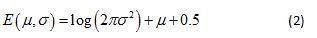
(see Appendix for the mathematical derivation of Eq. 2). In the analyses that follow, E (µ,σ) is computed for each week of the patient’s activity data using parameter estimates computed from the best-fitting lognormal multifractal spectrum.
Although no previous studies have applied multifractal analysis to activity data acquired from a subject susceptible to manic episodes, actigraphy measures have been analysed by the multifractal Hurst function, the precursor of the multifractal spectrum, to assess the effectiveness of light therapy for people suffering from Seasonal Affective Disorder [21]. For those who responded to the light therapy, the Hurst exponent decreased significantly suggesting multifractality, but the effect was quite small. Application of multifractal analyses to EEG data has shown that the peak location of the multifractal spectrum decreases as the level of consciousness increases from deep sleep to the awake state [22]. According to the Gaussian multiplicative cascade model, this result implies that the mean is inversely related to the level of consciousness during sleep.
The literature has shown different effects of pathology on the width of the multifractal spectrum. Whereas spectrum width measured using extracranial EEG data is greater for epileptics than for healthy individuals [23], studies using physiological measures such as heart-rate have shown that people with pathological conditions such as congestive heart failure produce multifractal spectra with considerably reduced width when compared with healthy individuals [24]. It is predicted that as a manic episode approaches for a person diagnosed with Bipolar I Disorder, a reduction in multifractal spectrum width will occur, possibly resulting from a decrease in the variance of a Gaussian multiplicative cascade model.
Testing for the presence of nonlinearity in activity time series
The importance of measuring the nonlinearity of data acquired from people diagnosed with a mental illness has been emphasized [25]. To detect nonlinearity in activity data, surrogate comparison series are obtained by computing the power and phase spectra of the original data series, randomly permuting the phase spectrum components and using the inverse Fourier transform to produce a new time series. This time series has the same statistical properties as the original time series in terms of its mean, variance, pdf and autocorrelation function, but without any dynamic nonlinearity [26].
For each transformed activity time series, 30 surrogate comparison series were generated using the TISEAN surrogates routine [27]. Evidence for nonlinearity based on the generalized Hurst functions was provided by comparing functions produced by the original activity data with a comparison mean generalized Hurst function computed using the surrogate data, each surrogate mean estimate being accompanied by its associated 95% confidence interval [5].
As an additional control, 30 normally distributed samples containing the same number of observations, and the same mean and variance as the data series were computed. Generalized Hurst functions with their associated 95% confidence intervals and multifractal spectra were computed for these normally distributed samples. It was expected that such series would be monofractal with the Hurst function being equal to 0.5 when q = 2.
Estimating change points in a time series
A commonly employed statistical technique for detecting change points in a time series estimates future values of the series based on a small number of previous values. If the prediction error becomes too large, a change in the parameters governing the time series will have occurred. The method used for this analysis, a semiparametric change detection procedure, can be accessed from commands available in the sac R package [28,29]. In this application, the cumsum.test command in sac with the “epidemic” option was used to detect two or more change points, and the schapt command was used to compute a semiparametric empirical likelihood ratio test from which the probability associated with the null hypothesis of no change could be computed.
The transformed activity data shown in Figures 2, 3 and 4 are for Week 9, when the Bipolar I subject appeared to be in a relative euthymic phase, and for Week 14, when the manic episode was fully developed and hospitalisation was imminent. Owing to a small amount of missing data, the multifractal spectrum parameters were not computed for Week 6.
All the other plots for Weeks 1 to 8 and Weeks 10 to 13 are available in the Supplementary Materials associated with this paper.
Log-log power spectra
Figure 2 shows the original activity data and the log-log power spectrum recorded for Weeks 9 and 14. The best-fitting linear log-log power spectra had slope estimates of –0.96 ± 0.03 and –1.03 ± 0.03 for Weeks 9 and 14, respectively. As there was no significant autocorrelation observed in the slope measures for each of the 14 weeks of the original activity data, a single sample t-test was used to support the null hypothesis that the overall mean slope was equal to –1, t(13) = –2.02, p>.05. This result confirmed the presence of pink noise in the untransformed activity data.
Figure 2. Raw activity data and log-log power spectra for (a) Week 9 and (b) Week 14. The best-fitting linear relationship between log power and log frequency is shown for the power spectra, together with the estimate and standard error of the slope.
Generalized Hurst exponent
The generalized Hurst exponent functions shown in Figure 3 were monotonic decreasing functions of q suggesting that the transformed activity data were multifractal. The functions for Weeks 9 and 14 estimated using the data (blue lines) were significantly different from those estimated using the surrogates (red lines) at all values of q except for q = 2, as indicated by the lack of overlap of the 95% confidence intervals. This finding was confirmed by the large Nonlinearity index, defined by the mean standard score difference between the data and surrogate points, the value of the index being 84.26 for Week 9 and 58.22 for Week 14. So the transformed activity data are nonlinear for all values of q except when monofractal DFA is applied with q =2. This finding shows the value of computing a complete multifractal analysis of these data rather than using DFA alone.
The green curves in Figure 3 show the generalized Hurst functions estimated from normal distributions with mean and variance equal to those of the transformed activity data. The 95% confidence intervals are shown for each point. For weeks 9 and 14, the data function deviated significantly from that generated by the normal distributions indicating that the data were not generated by a normally distributed process that occurred on a single time scale. Although there was no overlap between the data and control curves for Week 9, there was some overlap for q ≤ –3 for Week 14. Clearly the data were not samples from a normal distribution as the NonGaussian index, defined by the mean standard score difference between the data and normally distributed control points, was 40.10 in Week 9 and 21.93 in Week 14. It is worth noting that compared with the values for Week 9, the Nonlinearity and NonGaussian indices were both less for Week 14, suggesting a loss of nonlinear complexity in transformed activity scores between Weeks 9 and 14.
As shown in Figure 3, estimates of the Hurst exponent obtained from a monofractal DFA analyses of 0.18 and 0.23 for Weeks 9 and 14 respectively, were obtained from the generalized Hurst exponent functions when q = 2. The Hurst exponents for the corresponding surrogate series were 0.17 and 0.22, almost the same values as those estimated from the data. Hurst exponents less than 0.5 indicate that the differenced activity values were antipersistent, which is characterised by short duration runs of activity change in either the positive or negative direction rather than long runs of positive or negative differences. These Hurst exponent values were substantially different from the 0.51 obtained for the normally distributed control series for Weeks 9 and 14. A Hurst exponent equal to 0.5 is expected theoretically for a normally distributed process irrespective of its mean and variance.
If only a monofractal test such as DFA were applied to these activity data, as is common practice [12,13], there would have been no evidence for nonlinearity in the transformed activity data as the values of the Hurst exponent for the data and surrogate series were almost coincident. A multifractal analysis is required to obtain any useful information about nonlinear processes that might be responsible for generating activity data in humans, as is shown by comparing the data curve in Figure 3 with curves generated by the surrogate and normally distributed control series.
Figure 3. Generalized Hurst Exponent functions for (a) Week 9 and (b) Week 14 estimated using cubic detrending. The function for the transformed data (blue) indicates nonlinearity when there is no overlap with the 95% confidence intervals for the function computed using the surrogates (red) and the function generated by a normally distributed random variable with the same mean and variance as the transformed activity data. The Nonlinearity index is the mean difference between the data curve and the surrogate curve in standard normal distribution units. The NonGaussian index is the mean difference between the data curve and the curve generated from the normally distributed data in standard normal distribution units. The numbers in brackets are the DFA exponents for the data, surrogate and normally distributed control series respectively, estimated when q = 2 as shown by the vertical line.
Multifractal Spectra
Figure 4 shows the fit of the Gaussian multiplicative cascade model to the multifractal spectra estimated for Weeks 9 and 14 using Eq. (1). The fit of the model shown by the blue line was reasonably good, the peak location of the estimated multifractal spectrum being close to the mean of the lognormal distribution in each case (0.46 for Week 9 and 0.39 for Week 14). The width of the multifractal spectrum was positively related to the standard deviation of the Gaussian, being 0.64 in Week 9 and decreasing to 0.47 as the manic episode became imminent during Week 14.
Figure 4. Multifractal spectra for (a) Week 9 and (b) Week 14 estimated using cubic detrending. The blue line shows the best-fitting multifractal spectrum estimated using a multiplicative cascade driven by a Gaussian pdf. The data points are shown as small blue circles. The spectra estimated from the surrogate series and the normally distributed control series are shown by the red and green curves, respectively. The lognormal parameter estimates for µ and σ are shown in brackets at the bottom of each graph together with an estimate of the continuous Shannon entropy for the lognormal distribution. The MSE for the fit of the lognormal spectrum is also shown.
As it was already shown for the generalized Hurst functions, there was clear separation between the multifractal spectra computed from the transformed activity data (blue line) and spectra computed from the surrogate series (red line) and the normally distributed control series (green line). As expected, the maximum value of these latter two curves occurred when the singularity index, α, was equal to the monofractal Hurst exponent and 0.5, respectively. Evidence for clear multifractality in the transformed activity data was shown by the substantially greater width of the multifractal spectra for the data when compared with the spectrum widths for the control series.
Figure 5 shows the estimates of entropy for the lognormal pdf for each Week, computed using Eq. (2). As the multifractal spectrum was not available for Week 6 due to missing data, a suitable approximation of entropy for Week 6 was obtained by estimating its value using the average of the µ and σ estimates for Weeks 5 and 7. This approximation provided estimates of entropy that could be used effectively to detect change across all 14 weeks of activity observations.
Using the change point detection procedure and assuming for all practical purposes a Type I error probability of 0.1, significant change was detected at Week 5, p = 0.011, and at Week 12, p = .085, as indicated by the dotted vertical lines in Figure 5. This result shows that this patient experienced three mood stages during the 14 weeks of activity measurement, Stage 1 being perhaps a recovery period from a previous relapse between weeks 1 and 4 and Stage 2 being a period of relative euthymia from Week 5 to Week 11. During Stage 3 from Week 12 onwards, the precursors of the manic episode that led to hospitalisation became evident. A practical application of this finding would be for the patient’s medical team to have been alerted to a possible deterioration in this patient’s condition around Week 12.
Figure 5. Continuous Shannon entropy computed from estimates of the mean and standard deviation of a lognormal pdf using transformed activity data collected over a period of 14 weeks prior to the patient’s hospitalisation. The vertical lines show significant changes in entropy that occurred at Week 5 (p = .013) and at Week 12 (p = .085), with the Type I error probability set at 0.1 due to the relatively high cost associated with a Type II error in this preventative mental health application. The curve fit to the data points was estimated using a Lowess smoothing procedure. Cubic detrending was used to estimate the multifractal spectrum from the transformed activity data.
2021 Copyright OAT. All rights reserv
In this study, a unique prospective actigraphy dataset was interrogated for evidence of changes in complexity preceding a manic relapse. Analyses provided novel evidence for ‘hidden signals’ of the mania prodrome in high resolution objective time series data. First, we found that the relative invariance of the slopes of the log-log power spectra provided no useful predictive information about the imminent manic episode that occurred at the end of Week 14. It is worth noting that the pink noise detected for the patient in this study confirms a log-log spectrum slope of –1 obtained in previous analyses of mood rating data obtained from people diagnosed with bipolar disorder [30], although sometimes a more negative slope closer to –2 has been obtained for chronic depression [31]. Although slopes close to –1 suggest long-term correlations in the activity data, often associated with a complex time-scale invariant process, a more detailed multifractal analysis of these data offered greater insight into the temporal structure of activity data to facilitate its application in preventative mental health.
For the first time, we have shown that activity data recorded over an extended time period for a patient on the verge of a manic episode are clearly multifractal. Of considerable interest, the multifractal spectra could be predicted by a multiplicative cascade process driven by a Gaussian distribution with constant mean and variance. The predicted multifractal spectrum fit the data spectrum reasonably well, leading to estimates of the mean and standard deviation of the Gaussian that could be used to compute the continuous Shannon entropy for the related lognormal pdf. Application of change detection methodology revealed three stages during the 14 week observation period. The first stage represented a period of low but increasing entropy. The second stage revealed the highest entropy indicating a period of relative euthymia. The final stage was characterised by a dramatic decrease in entropy. As would also be the case for a number of chronic physical disorders, a decrease in entropy might signal the onset of deterioration in a patient’s mental health.
The change in multifractal spectrum complexity as the manic episode approached has a precursor in findings that EEG multifractal spectrum complexity, as indicated by spectrum width, increased prior to an epileptic seizure (preictal phase) and decreased dramatically as seizure activity increased. Compared with values estimated before and after reports of pain, multifractal spectrum complexity was less during periods of pain [32].
Perhaps multifractal spectrum complexity is greater during well periods than at times when a person with a dynamic condition such as bipolar disorder is euthymic. In the test case considered in detail in this paper, the reduced complexity of the multifractal spectrum may indicate that the usual feedback mechanisms that facilitate human-environmental interaction are disrupted as bipolar patients become unstable leading to an inability of the brain regulatory systems to properly manage mood [18,33].
When considered in terms a practical decision-making strategy for assessing the risk of a manic episode, the false alarm probability of 0.085 has considerable practical significance. If the algorithms described in this paper were used in a mobile monitoring device, the patient’s mental health team would be well-advised to check the patient’s current status when the chance of relapse by Week 12 was reasonably high. Those concerned with the huge costs involved in hospitalisation of patients with a serious mental health problem lasting several weeks if not months, would much prefer the minimal cost of preventative intervention by the medical and community mental health team to the immense cost of long-term hospitalisation. In Europe the average cost of inpatient hospitalisation for a person diagnosed with a manic episode in 1999 was €27297 per patient, the average stay being 47 days [34, Table V, p. 283]. This is a considerably greater relative cost than the average €169 required to assess a person’s mental health status, say at Week 12 for the patient discussed in the present paper, assuming such intervention circumvented hospitalisation.
If confirmed in future analyses of similar data from bipolar patients, these findings will allow medical intervention to occur well before the highly disrupted sleep that was observed about five days before the manic episode occurred [4]. Any automated device based on the findings for this patient will serve as a valuable contribution towards an improved standard of care for people diagnosed with bipolar disorder.
Evidence for nonlinear processes in the activity data were revealed by the significant discrepancies between generalized Hurst functions computed using the transformed data and functions estimated from surrogate series that had the same linear properties as the data but without the nonlinearity. This finding emphasises the advantage of using an objective measure such as activity rather than a subjective measure such as mood ratings [35-37], as well as technology that provides a more comprehensive account of the important multiplicative temporal interactions that might determine mood variation.
The use of actigraphy for predicting dynamic fluctuations in potentially psychopathological behavior may be more generally applicable than is evident at first sight. An interesting small-world network analysis of the contagion of all diagnoses contained in DSM-IV TR produced four diagnostic hubs, insomnia, with 71 connections to other symptoms, psychomotor agitation (68 connections), psychomotor retardation (61 connections) and depressive mood (60 connections) [38]. These four diagnostic hubs subsume 208 other symptoms in DSM-IV as well as 69 separately described disorders, a massive compression of diagnostic information (see Table 1 in [39]). Of considerable interest, all four diagnostic hubs can be assessed using actigraphy. Hence the technology proposed in this paper, which complements the Bipolar Vulnerability Index described in [40], may have wide application for monitoring substantial tracts of psychopathology space.
The defensible and effective mathematical analyses presented here is only one approach to complexity in manic relapse, and we are happy to share our data to encourage comparison. Data transfer from modern lifestyle monitoring devices using Bluetooth allows them to track complex psychomotor disturbance, even when the patient is relatively inactive during the highly diagnostic night-time hours [4]. An urgent challenge is to develop software for the mobile device so that the method used in this paper can be implemented in real-time.
Activity data acquired from a young male diagnosed with bipolar disorder over a long period of 14 weeks showed that, whereas there was no change over time in the monofractal nature of activity, multifractal spectra revealed significant changes in complexity that might serve as useful predictors of a future manic episode. As the analyses were based on a single manic relapse in a single patient, the generalizability of the findings is uncertain.
Nevertheless, it is rare to obtain so much continuous activity data over such a long period of time and we know of no other available data set. Unlike the design used in [41], there was no opportunity to track activity during hospitalization and subsequent recovery due to removal of the actiwatch as part of the admission procedure. In future studies we will request that an actiwatch or similar device be worn at all times.
The authors report no competing interests. The data for this study were collected at Swinburne University of Technology by the second author. The project was supported by a grant from the National Depression Initiative - beyondblue Centre of Research Excellence Project Grant to Professor G. Murray and Professor F. Judd. The data analyses were conducted by the first author. The writing of this paper was equally shared between the two authors. We acknowledge the significant contribution to this study by the subject who provided 103 days of actigraphy data despite his illness.
- Merikangas KR, Jin R, He JP, Kessler RC, Lee S, et al. (2011) Prevalence and correlates of bipolar spectrum disorder in the world mental health survey initiative. Arch Gen Psychiatry 68: 241-251. [Crossref]
- Grunze H (2010) The treatment of mania. In: Young AH, Ferrier IN, Michelak EE (Eds.), Practical management of bipolar disorder. Cambridge, UK: Cambridge University Press. 10-23.
- Lam D, Wong G (2005) Prodromes, coping strategies and psychological interventions in bipolar disorders. Clin Psychol Rev 25: 1028-1042. [Crossref]
- Bullock B, Judd FK, Murray G (2014) Using actigraphy to monitor sleep-wake patterns in bipolar disorder: a case study. Clinical Psychology Forum 253: 37-41.
- Heath RA (2000) Nonlinear dynamics. Techniques and applications in psychology. Mahwah, NJ: Lawrence Erlbaum Associates.
- Heath RA (2004) Complexity and mental health. In: Holt T (Ed.), Complexity for clinicians. Oxford, UK: Radcliffe Medical Press. 83-94.
- Murray G (2010) Circadian and sleep/wake considerations in the practical management of bipolar disorder. In: Young AH, Ferrier IN, Michelak EE (Eds.), Practical management of bipolar disorder. Cambridge, UK: Cambridge University Press. 152-162.
- Zelazny K, Simms LJ (2015) Confirmatory factor analyses of DSM-5 posttraumatic stress disorder symptoms in psychiatric samples differing in Criterion A status. J Anxiety Disord 34: 15-23. [Crossref]
- Ancoli-Israel S, Cole R, Alessi C, Chambers M, Moorcroft W, et al. (2003) The role of actigraphy in the study of sleep and circadian rhythms. Sleep 26: 342-392. [Crossref]
- Delignières D, Torre K, Lemoine L (2011) Methodological issues in the application of monofractal analyses in psychological and behavioral research. In: Guastello SJ, Gregson RAM (Eds.), Nonlinear dynamical systems analysis for the behavioral sciences using real data. Boca Raton, FL: CRC Press. 559-582.
- Mandelbrot BB (1997) The fractal geometry of nature. New York: Freeman.
- Hu K, Ivanov PCh, Chen Z, Hilton MF, Stanley HE, et al. (2004) Non-random fluctuations and multi-scale dynamics regulation of human activity. Physica A 337: 307-318. [Crossref]
- Yamahara M, Noguchi T, Okawa M, Yamada N (2009) The relationship between subjective sleep disturbance and complexity of 24-hour activity utilizing fractal theory in psychiatric inpatients. Sleep Biol Rhythms 7: 11-16.
- Kelty-Stephen DG, Palatinus K, Saltzman E, Dixon JA (2013) A tutorial on multifractality, cascades, and interactivity for empirical time series in ecological science. Ecol Psychol 25: 1-62.
- Kantelhardt JW, Zschiegner SA, Koscielny-Bunde E, Bunde A, Havlin S, et al. (2002) Multifractal detrended fluctuation analysis of nonstationary time series. Physica A 316: 87-114.
- Ihlen EA (2012) Introduction to multifractal detrended fluctuation analysis in matlab. Front Physiol 3: 141. [Crossref]
- Dean CB, Nielsen JD (2007) Generalized linear mixed models: a review and some extensions. Lifetime Data Anal 13: 497-512. [Crossref]
- Ihlen EA, Vereijken B (2013) Multifractal formalisms of human behavior. Hum Mov Sci 32: 633-651. [Crossref]
- Ashkenazy J, Havlin S, Ivanov PC, Peng CK, Schulte-Frohlinde V, et al. (2003) Relation between magnitude series correlations and multifractal spectrum width.
- Calvert L, Fisher A, Mandelbrot B (1997) Large deviations and the distribution of price changes. Cowes Foundation Discussion Paper No. 1165. New Haven, CT: Yale University.
- Ohashi K, Yamamoto Y, Teicher MH (2014) Locomotor microactivities associated with therapeutic responses in patients with seasonal affective disorders. Integr Med Int 1: 151-161. [Crossref]
- Torick T, Mandelkern MA (2013) Multifractal Detrended Fluctuation Analysis of human EEG: Preliminary investigation and comparison with the Wavelet Modulus Maxima Technique. PloS One 8: e68360. [Crossref]
- Dutta S, Ghosh D, Samanta S, Dey S (2014) Multifractal parameters as an indication of different physiological and pathological states of the human brain. Physica A 396: 155-163.
- Ivanov PC, Amaral LA, Goldberger AL, Havlin S, Rosenblum MG, et al. (1999) Multifractality in human heartbeat dynamics. Nature 399: 461-465. [Crossref]
- Bystritsky A, Nierenberg AA, Feusner JD, Rabinovich M (2012) Computational non-linear dynamical psychiatry: a new methodological paradigm for diagnosis and course of illness. J Psychiatr Res 46: 428-435. [Crossref]
- Schreiber T, Schmitz A (2000) Surrogate time series. Physica D 142: 346-382.
- Hegger R, Kantz H, Schreiber T (1999) Practical implementation of nonlinear time series methods: The TISEAN package. Chaos 9: 413-435. [Crossref]
- Guan Z (2004) A semiparametric changepoint model. Biometrika 91: 849-862.
- Guan Z (2009) The sac package. Version 1.0. Downloaded on 30 October 2015 from http://ftp.auckland.ac.nz/software/CRAN/doc/packages/sac.pdf
- Gottschalk A, Bauer MS, Whybrow PC (1995) Evidence of chaotic mood variation in bipolar disorder. Arch Gen Psychiatry 52: 947-959. [Crossref]
- Heiby EM, Pagano IS, Blaine DD, Nelson K, Heath RA (2003) Modelling unipolar depression as a chaotic process. Psychol Assessment 15: 426-434.
- Dick OE, Svyatogor IA (2012) Potentialities of the wavelet and multifractal techniques to evaluate changes in the functional state of the brain. Neurocomputing 82: 207-215.
- Both F, Hoogendoorn M, Klein CA, Treur J (2015) A generic computational model of mood regulation and its use to model therapeutic interventions. Biologically Inspired Cognitive Architectures 13: 17-34.
- Olié JP, Lévy E (2002) Manic episodes: the direct cost of a three-month period following hospitalisation. Eur Psychiatry 17: 278-286. [Crossref]
- Moore PJ, Little MA, McSharry PE, Geddes JR, Goodwin GM (2012) Forecasting depression in bipolar disorder. IEEE Trans Biomed Eng 59: 2801-2807. [Crossref]
- Moore PJ, Little MA, McSharry PE, Goodwin GM, Geddes JR (2014) Mood dynamics in bipolar disorder. Int J Bipolar Disord 2: 11. [Crossref]
- Ortiz A, Bradler K, Garnham J, Slaney C, Alda M (2015) Nonlinear dynamics of mood regulation in bipolar disorder. Bipolar Disord 17: 139-149. [Crossref]
- Borsboom D, Cramer AO, Schmittmann VD, Epskamp S, Waldorp LJ (2011) The small world of psychopathology. PLoS One 6: e27407. [Crossref]
- Hu K, Scheer FA, Ivanov PCh, Buijs RM, Shea SA (2007) The suprachiasmatic nucleus functions beyond circadian rhythm generation. Neuroscience 149: 508-517. [Crossref]
- Indic P, Salvatore P, Maggini C, Ghidini S, Ferraro G, et al. (2011) Scaling behavior of human locomotor activity amplitude: Association with bipolar disorder. Plos One 6(5): e20650.
- Krane-Gartiser K, Henriksen TE, Morken G, Vaaler A, Fasmer OB (2014) Actigraphic assessment of motor activity in acutely admitted inpatients with bipolar disorder. PLoS One 9: e89574. [Crossref]