Take a look at the Recent articles

Abstract

Despite numerous policy initiatives and major economic transformations, India has one of the highest rates of child malnutrition in the world. This paper examines the effect of women’s autonomy within the household on child nutritional outcomes. In addition, it also examines the effect of public spending on nutritional outcome as well as in improving women’s autonomy.

Data from two cross-sectional waves of the National Family and Health Survey (1998-99 and 2005-06) were used. The measures for malnutrition were the height for age standardized score and stunting; the measure of public spending was state-level expenditure in social sectors; and the measure for women’s autonomy was an index based on evidence of decision-making, sources of such power, and contexts of such power. The statistical analyses using multivariate regressions show that women’s autonomy has a significant positive effect on child nutritional outcomes, particularly in cases of severe malnutrition and in states with a high prevalence of stunting. Public spending on development and welfare has a significant effect on nutritional outcomes, with a stronger effect in states that have a high prevalence of malnutrition. In addition, public spending in the social sector has a significant effect on increasing autonomy within the household.

The results indicate the importance of women’s autonomy on child nutritional outcomes in the context of other instruments of public policy, as well as the role of public expenditure in improving women’s autonomy in addition to its direct role in improving nutritional outcomes. The study highlights the complementarity of different elements of public spending in achieving development goals.

Key words

epidemiology, prescribing indicators, patient care indicators, facility indicators, diabetes, southern punjab region

Introduction

In the last few decades, India has made significant progress in reducing early childhood malnutrition. The proportion of children with chronic malnutrition in rural areas went down from 79% to 52% between 1975-79 and 2003-06 [1,2]. The proportion of children (under 3) with chronic malnutrition went down from 53% to 45% between 1992-93 and 2005-06 (authors calculation from National Family Health Survey [3], though the decline was less in rural areas than in urban areas. However, the levels are very high by international standards. The proportion of children under 5 with chronic malnutrition at 43% in 2006 is significantly higher than the world average (31%), the average for developing countries (32%) and even countries in Sub-Saharan Africa (38%) [4]. A recent study by the International Food Policy Research Institute, ranked India 117 among 119 countries in child malnutrition [5]. Malnutrition remains a problem despite numerous policy initiatives specifically targeting malnutrition and major economic transformation resulting in significant reduction in poverty in recent years [6,7].

The main reasons for malnutrition are inadequate intake of calories, protein, and micronutrients, as well as diseases that reduce the body’s ability to absorb and process nutrients [8] and often it is irreversible [9,10]. Malnutrition has serious consequences on mortality, morbidity, and human development [11]. In developing countries, malnutrition is responsible for at least a third of deaths among children under five [12-14]. In addition, it affects development of the brain and the central nervous system affecting evolution of motor skills and cognitive development [15]. These have important consequences on school preparedness, late enrollment, and dropout rates and educational attainment [16-19]. India ranks 54 in under-five mortality with mortality at 74 per thousand live births in 2005 and account for nearly a quarter of the 7.2 million under five deaths globally [20]. Average years of schooling among the 15+ population is less than five years, and though there is near-universal enrollment at the primary level, almost half the students drop out of schools by the secondary level [21].

Formal modeling of malnutrition by Maxwell and Smith [22] identifies insufficient access to food, inadequate maternal and childcare practices, poor water and sanitation, and inadequate healthcare services as the underlying causes of malnutrition among children. Further, all of these underlying causes are affected by the quantity and quality of actual resources within the household and how they are controlled.

A variety of economic models of household that focus on differences in preferences among its members [23]. Himmelweit, et al. [24] observe that the relative bargaining power of its members plays an important role in determining the allocation of resources within the household towards private (e.g. own consumption and health) and public (e.g. children) goods. The source of such a bargaining power is usually attributed to the resources controlled by each member. In addition, it is also influenced by social norms, interpersonal network and attitudes [25].

In developing countries, women are involved in most of the underlying causes identified in the model by Maxwell and Smith. Thus, they are likely to be in a better position to take decisions, that have consequences on child nutritional outcome [26]. In such circumstances, access to resources and ability to take decisions regarding allocation of resources has important consequences on effective care-giving and child health outcomes.

Due to several reasons (property rights, low participation in paid work, cultural factors, among others) status of women in India within the household as well as the society in general is low compared to women in other developing countries [27]. India ranks 122 among 138 countries in the Gender Inequality Index based on conditions in reproductive health, empowerment, and labor market participation [28]. Ramalingaswami, et al. [29] observe that countries in South Asia have a poorer nutritional outcome than countries in Sub-Saharan Africa even though they are better off than the latter in terms of per capita GDP, per capita dietary energy supply, and access to safe water. They argue that the difference is mainly because of the low status of women in South Asia, as Sub-Saharan countries have better female-to-male life expectancy, female literacy rates, and women’s share in the labor force and earned income.

Though household allocation is immensely important, the role of other factors like poverty plays a much more important role in developing countries like India. Food comprises approximately half of total household consumption expenditure and nearly three-fourth for those in the lowest income quartile in India [30]. In addition, poverty affects health inputs and provision of household infrastructure like water and sanitation.

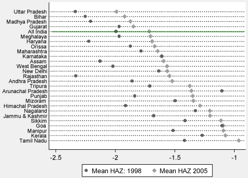
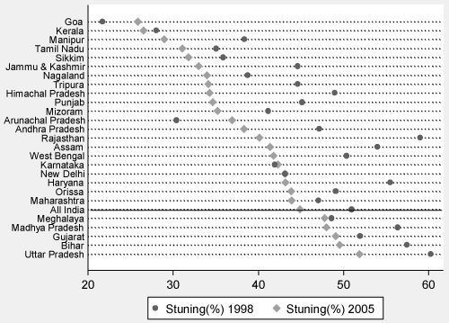
A related issue is the high level of variation in malnutrition across Indian states. In the last two surveys of National Family Health Survey (1998-99 and 2005-06), the all-India average for height for age standardized z-scores (HAZ) (a measure of chronic or long-term malnutrition) was -1.99 and -1.71 respectively (for children less than 3). In three states – Bihar, Madhya Pradesh and Uttar Pradesh – the average HAZ was lower than the national average in both periods (Figure 1) Gujarat, which had average HAZ slightly above the national average in 1998 declined to lower than the national average by 2005. Four states, Assam, Haryana, Rajasthan, and West Bengal improved from being lower than the national average to higher. There are 18 states that had higher than average levels of HAZ in both periods. The same 18 states had higher than average prevalence of stunting (when HAZ is 2 standard deviation below the average of relatively healthy children) (Figure 2) with the exception of Meghalaya, which had higher than average proportion of stunting in 2005 and West Bengal which, despite lower than average HAZ in 1998, managed to have lower than average stunting in both periods. The three states that had lower HAZ in both periods also had a higher prevalence of stunting. In addition, Gujarat had higher than average stunting in both periods. The proportion of stunting declined in Assam, Haryana and Rajasthan between the surveys.

Figure 1. Mean HAZ by States for children under 3 years of age

Figure 2.Percent Stunting by States for children under 3 years of age

Economic growth through its impact on poverty may have significant effects on malnutrition. Given the nature of the states with persistent malnutrition, one may be tempted to correlate lack of economic growth with malnutrition. However, it is difficult to make such generalization as we can also see that states like West Bengal which showed improvements between the surveys was one the states with very little economic growth during the period, while states with very high level of growth in recent years, like Gujarat actually performed poorly in terms of malnutrition.

A recent study on malnutrition in India by Subramanyam, et al. [31] found that economic growth at the state level had no impact, while Pathak and Singh [32] found that growing inequality has adversely affected malnutrition. For economic growth to affect the living conditions of poor, it requires that the asset base of the poor household should be developed enough to participate in the growth process and the growth needs to be intensive in assets they hold and in sectors, they dominate [33]. Situation for such inclusive growth varied widely among the different states, part of which is due to the nature of public spending among them [34].

The other possible source of such state-wide variation is the level of public spending towards child health and nutrition. Public programs can play an important role in addressing high levels of malnutrition, particularly when economic growth is not sufficient [35]. However, the literature on public spending on health in developing countries [36-39] is not conclusive as to whether public spending can have a significant effect on health outcomes.

Filmer, et al. [40] identify two main problems – difficulty in converting public expenditure to effective services and the problem of crowding out of private services – which results in limited effect of public expenditure on health and related outcomes. In addition, India spends a very low share of its gross domestic product on social sector expenditure, which results in poor and inadequate coverage [41]. Even then, several India- specific studies find a significant effect of public spending on child mortality among vulnerable population in poor states or rural areas [42-44].

In the case of malnutrition, however, the evidence is not encouraging. The most important public program towards nutritional outcomes in India is the Integrated Child Nutritional Services (ICDS) set up in 1975. A study by Lokshin, et al. [45] find no significant effect of the program on child nutritional outcome. Gragnolati, et al. [6] identifies several limitations of the program which may explain such limited impact. They find that main focus of the program regarding nutritional outcome was towards food-based intervention ignoring other determinants of malnutrition. Also, even though most of the manifestation of childhood malnutrition takes place before the age of three, the program directed nutritional supplementation for children in ages four to six years ignoring earlier age groups. In addition, targeting was poor, specifically for children from socially disadvantaged groups like those from poor families or low caste. Besides under the program states with highest prevalence had the lowest funding and coverage.

The primary objective of this paper is to examine whether women’s autonomy within the household has significant effects of malnutrition in India. By “autnomy” here I refer to an individuals “capacity to control one’s personal environment” as discussed in Dyson and Moore [46]. Further, I examine the role of public expenditure and economic growth to promote both nutrition and women’s autonomy. Several studies [47] (for review of empirical research) have looked into the relation between indirect measures of autonomy like maternal education, height, or possible sources of bargaining power, e.g. earned income and asset at marriage and resource allocation. Though Ramalingaswami, et al. [29] indicated the relevance of the relation there are very few published research, which explores the role of autonomy in a representative sample for India. A couple of studies by Smith and coauthors [48,49] did address this, but their studies did not consider actual decision making but they restricted measure of autonomy to sources and settings of such power. Studies with wider sets of measures [50]. Shroff, et al. [51] for rural areas of a single state in India and Mabsout and Van Staveren [52] however, do not explore the role of economic condition and public expenditure in shaping women’s autonomy.

Given the high prevalence of malnutrition in India, it is necessary to reconsider the policy alternatives. Instead of concentrating on specific programs to improve outcomes, there is a need to take a systems approach to the problem. The study by Lokshin, et al. [45] observed that even though the ICDS program had no significant effect on malnutrition, it was more successful in areas where there was a significant amount of ongoing development programs. This indicates the synergistic nature of different elements of public spending.

A significant amount of literature indicates that women’s autonomy plays an important role in the nutritional outcome, but there is very little effort in India to operationalize autonomy as a policy instrument. This is where public spending can potentially play an important role in influencing the sources and settings of their decision making abilities. Beyond that, public spending can play important roles by translating economic growth to poverty reduction and addressing regional imbalances of market based growth.

Data and Methods

Data

In this study, I use data from two rounds of the National Family and Health Survey conducted during 1998-99 (NFHS-II) and 2005-06 (NFHS-III). These cross-sectional, nationally representative household survey data have relevant information on child nutritional status as well as instruments that can be used to construct a measure of mother’s autonomy within the household [3]. The NFHS is part of the Demographic and Health Surveys conducted in several developing countries across the world [53]. Though all the surveys have similar instruments, some of the relevant questions on women’s decision making were introduced in NFHS-II. In addition, anthropometric measures were not collected for several states in the earlier survey. I use economic indicators and public finance data from the Handbook of Statistics on State Government Finances [54].

Analytical model

In this paper, I discuss malnutrition in terms of height for age standardized z-scores (HAZ) which is a measure of chronic or long-term malnutrition. In addition, I use two measures derived from HAZ – stunting where the child has HAZ less than negative two (or less than two standard deviations from the mean value of zero), and severe stunting where HAZ is less than negative three.

I assume that child nutritional outcome is a result of household optimization. Parents optimize their utility from own consumption and leisure and utility derived from their child’s health. The choices are constrained by household budget and child health production function. Child health production involves health and related inputs, child and household characteristics. Autonomy enters the model in its ability to influence the production process. Additionally, it is assumed that macro-economic conditions like level of economic development, can affect the availability of heath and related inputs. Public spending is relevant when economic development is not sufficient.

This gives the basic reduced form relationship that I examine using multivariate regression methods

Child’s Nutritional outcome ~ f₁(Mother’s Autonomy Index, State Public Spending, State Economic Indicator, Child controls, Parental Controls, Household Controls, State and Year fixed effects)

In case of autonomy, I assume that variation in autonomy can be explained by woman and spouse characteristics, household characteristics and local-level factors, which can influence the sources and settings of autonomy (Kabeer, 1999). In addition, economic development and public spending in health, education and development can improve autonomy by improving both sources and settings of power.

To examine this, I consider the following reduced form relationship

Mother’s Autonomy Index ~ f₂(State Public Spending, Economic Indicator, Spousal controls Household Controls, Local controls, State and Year fixed effects)

The nutritional outcome that I examine here is HAZ, stunting and severe stunting based on the WHO median values [55]. Several studies have confirmed that these measures are reasonable for evaluating malnutrition in India [56,57]. For HAZ, I use ordinary least squares and quantile regression specifications. I estimate stunting and severe stunting using logistic regression models.

Perception of control in household decision making is the fundamental basis of measuring autonomy [58,59]. However, there are other aspects, which shape the bargaining process [52,60]. Particularly pre-existing gender norms can limit what is bargained over and whether someone is entitled to bargain and whether it is appropriate to bargain [61,62]. I create the autonomy index based on actual evidence of power (whether woman makes decision by herself or jointly on own health and major household item and visit to relatives or friend or that and whether they have money set aside for personal use), sources of power (whether woman work for cash, regular exposure to newspaper, radio and television) and settings in which power is exercised (the percent difference between woman and spouse’s age, the difference between woman and spouse’s years of education, whether the woman is in a non-nuclear family) including norms and attitudes (whether there is any reason for domestic violence, whether the woman desires more sons than daughters and age at first marriage). A single factor is created using an iterative principal factor analysis on the polychoric correlation between the different variables and is used to create and autonomy index, centered to vary between 0 and 100.

Table 1 shows the factor loadings and the distribution of the different components used in the construction of the autonomy index. The highest factor loadings are for decision on health and major household purchase followed by age at first marriage. Acceptance of any reason for domestic violence and son preference as well as belonging to non-nuclear family shows negative factor loadings. Due to the abstract nature of the index and the relative nature of the measure, I create three quantiles of the autonomy index – low, medium and high. The table shows that the main difference between the levels of the autonomy index is in decision making on health and household durables, followed by media exposure, and whether money is set aside for self. Important factors like age at first marriage and percent working for cash does not vary much, and they are generally low in case of India.

Table 1. Women’s Autonomy Index

	Factor loadings	Full Sample		Low Autonomy Index		Medium Autonomy Index		High Autonomy Index
			Yes		Yes		Yes		Yes
Decision on own health	0.659		56.4%		12.8%		64.6%		91.8%
Decision on household durables	0.663		51.7%		9.4%		56.7%		89.4%
Decision on movement	0.339		14.4%		6.1%		12.2%		24.9%
Money set aside for own use	0.333		47.3%		31.1%		45.9%		65.3%
Any reason for domestic violence	-0.170		49.5%		58.1%		50.4%		39.8%
Son preference	-0.269		29.2%		41.6%		29.8%		16.1%
Any media exposure	0.390		59.2%		38.0%		57.4%		82.9%
Works for cash	0.080		18.7%		17.5%		17.4%		21.0%
Non-nuclear family	-0.125		57.6%		63.3%		57.2%		52.6%
		Mean	Std Dev	Mean	Std Dev	Mean	Std Dev	Mean	Std Dev
Age difference with spouse (%)	0.122	-0.23	0.18	-0.26	0.20	-0.23	0.18	-0.18	0.15
Education difference with spouse (in years)	0.204	-2.12	4.15	-3.43	4.24	-2.26	4.05	-0.68	3.69
Age at first marriage	0.425	18.26	3.61	16.21	2.26	17.73	2.87	20.89	3.79

Earlier studies by Subramanyam, et al. [33] indicates that state level net domestic product has no explanatory power on malnourishment among children in India. Instead, I consider percent below poverty in rural areas as the measure of state level economic development. For measure of rural poverty, I use percent below the poverty line from the Planning Commission of India (30-day day recall of 1999-00 and Uniform Recall Period for 2004-2005).

There are three main components of state level social sector expenditure in India – expenditure on medical and public health (including expenditures on family welfare and health-related issues like water supply and sanitation and nutrition), expenditure on rural and urban development (including expenditure on welfare of backward caste, tribes and classes) and expenditure on education and related areas. To identify the role of public expenditure on the nutritional outcome, I consider the effect of state level social sector expenditure on development and welfare. Since there are annual fluctuations in public spending, and since the outcome of interest is a long term measure of malnutrition, I consider average expenditure for five years prior to the survey year. The choice of five years is motivated by five-year economic planning cycle as well as the election cycle in India, which are usually associated with policy shifts.

In addition to the above, I also control for child level variables like child’s age in months, sex and number of sibling; parental variables like mother’s age and education and father’s education and occupation; household head’s religion and ethnic (caste) characteristics, wealth index and environment factors like availability of piped water and flush toilets and location in rural as against urban areas. Further, I consider state fixed effects to control for unobserved state level characteristics as well as fixed effects for year of the survey.

The specifications for autonomy index are similar except that it does not contain any child controls, and it additionally controls for local (primary sampling unit) level proportion of mothers with son preference and those who work for cash and average years of education among mothers to address the effect of local institutions in determining women’s autonomy within the household [48]. Regressions are estimated using ordinary least square methods.

In the autonomy index specification, instead of only developmental expenditure, I consider all social sector expenditure as all of them can potentially affect autonomy. However, it is possible that there may be reverse casualty between autonomy index and social sector expenditure as more empowered women may demand higher level of public expenditure in the social sector through electoral participation or otherwise [63]. Furthermore, both autonomy index and state level social sector expenditure may be jointly determined by other factors like land tenure system during colonial times [64] or socio-economic and political configuration within states at the time of independence [65]. To address this, I instrument social sector expenditure using the proportion of state expenditure for the non-developmental purpose which mainly includes expenditure on interest payments on debt, salaries and pensions of government employees, administrative services, etc.

I adjust all nominal variables to 2006 Indian rupees using the Consumer Price Index for Agricultural Laborers [52]. Per capita figures were constructed using population projections from the Registrar General of India (Population Projections for India and States 1996-2016 and 2001-2026).

The total sample of children under three years of age with mothers who are married and usual residents of the household during the survey is 53,616. Keeping children who is singleton, results in a sample of 53,006 children. I further exclude children for whom anthropometric measures are outside of plausible limits or not available (4,259 or 8.03%). The regression for the nutritional outcome is conducted on 41,877 children after excluding 1,908 (4.36%) cases where right-hand side variables are not available. The anthropometric variables are not significantly different between those with missing right-hand side variable and those without. However, missing anthropometric variables are strongly related to most of the control variables. The regression for autonomy index is conducted on 37,714 mothers whose children are considered for the regression on the nutritional outcome.

Results

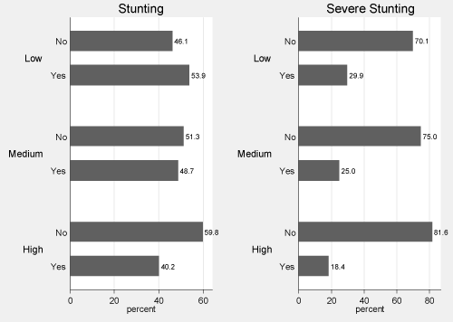
Figures 3 to 8 show the relation between the main variables. Figure 3 show that there is an inverse relationship between autonomy levels and proportion of stunting. The prevalence of stunting is highest among mothers with low autonomy level, and it declines significantly in the case of mothers with high autonomy. The decline in prevalence of autonomy is higher (38%) in case of severe stunting compared to stunting (25%).

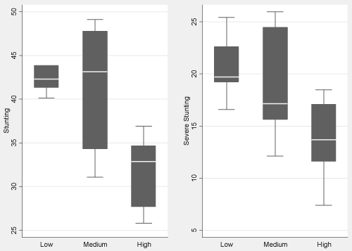
There is also a significant difference in prevalence of stunting at the state level between states with high and low levels of per-capita development expenditure. However, the states with medium level of per capita expenditure do not necessarily have low levels of stunting compared to low expenditure state, though in both cases of stunting they fared worse than the high expenditure states (Figure 4).

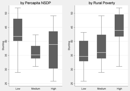
Figure 5 shows the distribution of stunting at the state level by per-capita Net State Domestic Product (NSDP) and by levels of rural poverty. In case of NSDP, though it improves between low and medium levels, average stunting is not necessarily low for high levels of NSDP. The inverse relationship between stunting is more obvious in case of rural poverty, though there is some overlap between states with low and medium levels of poverty.

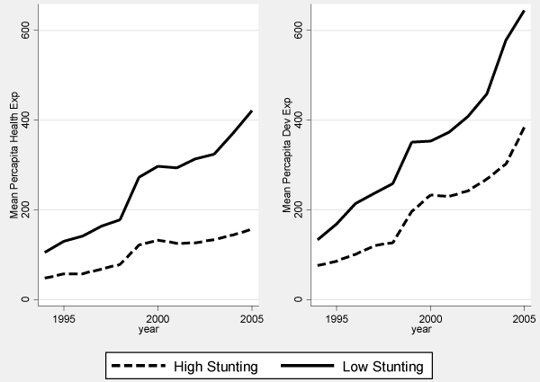
Figure 6 shows that per-capita expenditure on Medical and Public Health (from which fund is allocated for the ICDS and other programs) was generally flat over the period, except for a nudge just before 2000 for states with high prevalence of stunting. The behavior is unlike the states with low prevalence of stunting where it went up significantly over time. In case of development expenditure, it rises for high prevalence states, but the levels as well as the rates of the increase are much lower than the low prevalence states.

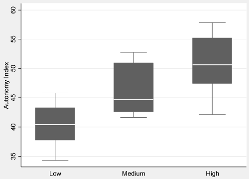
Figure 7 shows a very strong relation between average state level autonomy index and per capita social sector expenditure. Social sector expenditure can increase autonomy as each of the main components of the expenditure has potential association with sources and settings of power. Higher level of medical and public health expenditure, improve health care utilization and health literacy. Higher educational expenditure which in India’s case is often associated with higher past trends, can improve autonomy both through its intrinsic value as well as improving employment prospects. Developmental programs, particularly in rural development and welfare programs for underprivileged groups can create a more conducive environment for higher autonomy by improving movement, communication, labor-force participation, etc.

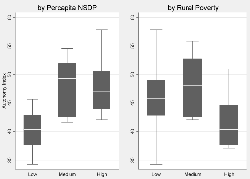
However, the relation between measures of economic development and autonomy is ambiguous both in case of per-capita NSDP and rural poverty (Figure 8). Though both low levels of NSDP and high level of poverty is associated with the lowest level of autonomy compared to medium levels, the highest level of NSDP and lowest level of rural poverty does not improve the level of autonomy.

Figure 3. Percent Stunting by Autonomy Index

Figure 4. Stunting by development expenditure, 2005

Notes: Average developmental expenditures for five years prior to the survey year.

Figure 5. Stunting by different measure of economic development, 2005

Notes: Average Net State Domestic Product (NSDP) for five years prior to the survey year.

Figure 6. Average Medical and Public Health expenditure and Developmental expenditure for states with high and low prevalence of stunting

Notes: A state is considered to be high prevalence, if the prevalence was higher than the national average in either of the NFHS surveys. West Bengal, which had lower prevalence in both surveys was also included as it had higher than average HAZ in the 1998 survey.

Figure 7. Autonomy by per capita social sector expenditure, 2005

Figure 8. Autonomy by different measure of economic development, 2005

Regression results

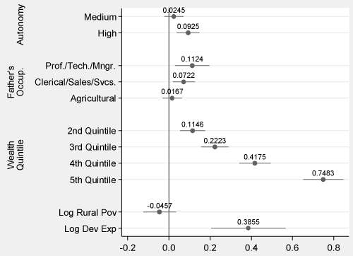
Results of the regression analysis on HAZ shows that HAZ declines significantly with child’s age and number of sibling. The results do not show the negative effect on child’s gender as I also control for the number of sibling which is an important mechanism through which gender bias affects child outcome [66]. Mother’s education plays a significant role. Father’s education and occupation which are also a proxy for income in this model significantly affects HAZ. Among religion and ethnic groups, Muslims and those belonging to the Scheduled Caste shows the worse outcome. The asset-based wealth index is highly significant. Among environmental factors, flush toilet plays a significant role, after controlling for income and assets. Even after controlling for these factors, autonomy index has a significant effect on HAZ levels. A 10 percent in the autonomy index increases HAZ by 2.85 percent points (pcpts). Specifications with and without autonomy index, does not change the coefficients of other controls except for mother and father’s education at the primary level and in case of rural residence. This would indicate that the effect of autonomy on HAZ is independent of other factors, specifically father’s occupation, household assets and household religion and ethnic groups.

Though the autonomy index has a significant effect on HAZ, when different levels of autonomy are considered, autonomy is only significant at higher levels (Figure 9). Belonging to the highest level of autonomy improves HAZ by 9.25 pcpts. Rural poverty does not have a significant effect on mean HAZ, but the level of developmental spending does. A 10 percent increase in developmental expenditure increases HAZ by 3.86 pcpts. It is important to note that in terms of magnitude, wealth differentials have the largest effect on HAZ. Compared to the lowest-income quintile, belonging to the second quintile increases HAZ by 11.46 pcpts and belonging to the highest quintile increases HAZ by 74.83 pcpts.

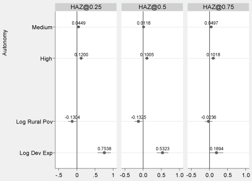
The results of quantile regression at different quantiles of HAZ show that autonomy has a stronger impact in increasing HAZ at lower quantiles. However, unlike the regression at the mean, the effect of rural poverty is significant at 25^th percentile and 50^th percentile. In all cases, the level of developmental expenditure is highly significant, though the effect of developmental expenditure is almost four times at 25^th percentile compared to at 75^th percentile (Figure 10).

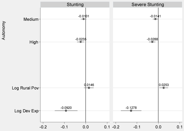
The results of the logistic regression show that for stunting, autonomy index has a significant effect only at higher levels though it is significant for both medium and high level of severe stunting. Developmental spending is significant in either case, but the marginal effects are larger in case of severe stunting. Rural poverty does not affect stunting but significantly increases the probability of severe stunting (Figure 11).

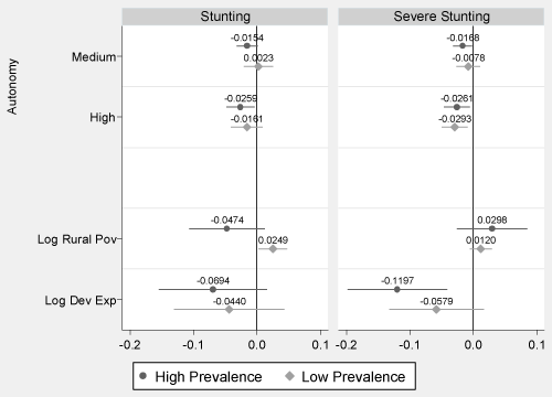
In states with a high prevalence of stunting, both medium and high autonomy levels significantly reduce the probability of stunting (Figure 12). The effect is not similar in the case of states with low prevalence of stunting where the effect is significant only at high autonomy levels and in case of severe stunting. Poverty increases the probability of stunting only in states with low prevalence (at 90% confidence level) and developmental expenditure significantly reduces the probability of severe stunting in states with high prevalence.

Regression on the autonomy index shows that autonomy increases with mother’s education. However, it decreases with father’s education, because women generally withdraw from the labor force [67,68]. Though the effect of autonomy is stronger for professional/technical/managerial occupations, it is worse for agricultural laborers. The scheduled tribes are not different from scheduled castes, but the other backward classes also show lower levels of autonomy which is also possibly due to withdrawal from the labor force [67]. Local factors, like social norms about son preference and labor-force participation show a significant effect on autonomy in the expected direction. In addition, rural location has a significant effect on autonomy compared to urban areas. The introduction of state level variables has a limited effect on other coefficients. Rural poverty levels significantly affect autonomy. A 10 percent decrease in rural poverty increases autonomy by 3.96 pcpts (Table 2). The negative and significant coefficient for developmental spending maybe due to endogeneity discussed earlier. Using the share of non-development expenditure in total state level expenditure as an instrument, I find that social sector expenditure has significant and substantial effect on autonomy index. Test of endogeneity rejects the null hypothesis of exogeneity of social sector expenditure on autonomy index. The coefficient for the excluded instrument is significant and the F statistic for the first stage regression is significantly higher than the rule of thumb value of 10.

Figure 9. Coefficients and 95% confidence interval for selected variables on HAZ

Notes: Other controls discussed in text.

Figure 10. Coefficients and 95% confidence interval for selected variables on HAZ for different quartiles of HAZ

Notes: Other controls discussed in text.

Figure 11.Marginal effects and 95% confidence interval for selected variables on Stunting and Severe Stunting

Notes: Other controls discussed in text.

Figure 12.Marginal effects and 95% confidence interval for selected variables on Stunting and Severe Stunting for states with High and Low Prevalence of Stunting

Notes: High and Low prevalence States are as defined earlier in Figure 6. Other controls discussed in text.

Table 2.Regression results for Autonomy Index

	OLS	Instrumental variable regression
		First Stage	Second Stage
	Autonomy Index	Log Percapita Soc.Sec.Exp.(5yr avg)	Autonomy Index
VARIABLES
Log Percent Below Poverty (Rural)	-3.956***	-0.00572***	-3.721***
	(0.3026)	(0.0010)	(0.3047)
Log Percapita Soc.Sec.Exp.(5yr avg)	-7.432***		34.94***
	(1.8521)		(13.0554)
Log Share of Nondev Exp		-0.0882***
		(0.0030)
Observations	37,715	37,715	37,715
R-square	0.332	0.995	0.318

Notes: Regression estimates controlled for mother and spouse characteristics, household and local characteristics, state and year fixed effects Robust standard errors in parentheses; ***p<0.01, **p<0.05,

*p<0.1, Durbin-Wu-Hausman, Robust regression F(1,37664) = 11.0714  (p = 0.0009), F statistic for joint significance of the instruments, F(1,37665) = 865.752 Prob > F=0.0000.

Conclusion

Women’s autonomy does have a significant effect on child nutritional outcome. However, the effects are significant only at higher levels of autonomy. Public spending on rural and urban development and welfare of socially disadvantaged groups has a significant positive effect on nutritional outcome. On the other hand, social sector expenditure has a significant positive effect on improving women’s autonomy. Poverty reduction does not have a significant effect on reducing moderate and severe stunting but has a significant effect on reducing severe stunting as well as improving women’s autonomy. Proxies for income like father’s education and occupation as well as the wealth index based on household assets has a significant effect on the nutritional outcome.

The use of HAZ and stunting as a measure of nutritional outcome has its limitations as there are several other aspects of malnutrition as those due to lack of micronutrients, which also have serious consequences [13]. The choice of HAZ is mainly due to its availability and the relative difficulty in obtaining other types of measures from regular surveys. It is very likely that protient-calorie malnutrition is generally correlated with micronutrient deficiencies though the effect of autonomy, public spending and poverty may differ. Several studies e.g. Filmer, et al. [40] and Rajkumar and Swaroop [69] have indicated the role of governance in the effectiveness of public program, and here I do not control specifically any measure of governance. However, assuming these characteristics does not change very rapidly in short period of time, they are implicitly accounted in the state fixed effects. It is important to recognize that it is difficult to measure autonomy [60,70] and the variable used here is merely an indicator of the main concepts highlighted in the literature. In this study, I use the measure of autonomy at the time of the survey as a proxy for autonomy during the lifetime. This implicitly assumes that autonomy index does not change significantly in short period of time, which is to a certain extent acceptable, but it may have its consequence on using autonomy as a policy instrument to address malnutrition.

This study raises two important issues in tackling childhood malnutrition in India, the role of woman’s autonomy and the role of public expenditure in reducing malnutrition and improving autonomy. In addition, it also highlights the importance of poverty reduction as against raising gross domestic product in addressing the malnutrition problem. This is particularly important since India has widespread malnourishment, and targeted programs may be costly and may have limited success [33,71,72]. Beyond that the results also highlight the complementarities of the different aspects of public spending in achieving desired outcomes.

References

<

1. National Nutrition Monitoring Bureau (1999) Report of the Second Repeat Survey - Rural. National Insitute of Nutrition, Hyderabad.
2. National Nutrition Monitoring Bureau (2008) Factsheets MND-Nutristatus. National Insitute of Nutrition, Hyderabad.
3. IIPS (2007) India National Family Health Survey (NFHS-3), 2005-06: International Institute for Population Sciences.
4. UNICEF (2007) The state of the world's children 2008: Child survival: Unicef.
5. von Braun J, Ruel M, Gulati A (2008) Accelerating Progress toward Reducing Child Malnutrition in India. International Food Policy Research Institute pp. 2-8.
6. Gragnolati M, Shekar M, Das Gupta M, Bredenkamp C, Lee Y (2005) India's Undernourished Children: A Call for Reform and Action. Nutrition and Population Working Paper, The World Bank. Washington, DC.
7. Tarozzi A, Mahajan A (2007) Child nutrition in India in the nineties. Economic Development and Cultural Change 55: 441-486.
8. Morris S (2001) Measuring nutritional dimensions of household food security. In Hoddinott J (Ed) Food Security in Practice: Methods for Rural Development Projects. International Food Policy Research Institute, Washington DC.
9. Martorell R (1999) The nature of child malnutrition and its long-term implications. Food and Nutrition Bulletin 20: 288-292.
10. Stein AD, Melgar P, Hoddinott J, Martorell R (2008) Cohort profile: The Institute of Nutrition of Central America and Panama (INCAP) nutrition trial cohort study. Int J Epidemiol 37: 716-720.
11. Grantham-McGregor S, Cheung YB, Cueto S, Glewwe P, Richter L, et al. (2007) Developmental potential in the first 5 years for children in developing countries. The lancet 369: 60-70.
12. Alderman H, Lokshin M, Radyakin S (2011) Tall claims: Mortality selection and the height of children in India. Economics & Human Biology 9: 393-406.
13. Black RE, Allen LH, Bhutta ZA, Caulfield LE, De Onis M, et al. (2008). Maternal and child undernutrition: global and regional exposures and health consequences. The lancet 371: 243-260.
14. Jones G, Schultink W, Babille M (2006) Child survival in India. Indian J Pediatr 73: 479-487. [Crossref]
15. Hoddinott J, Maluccio J, Behrman JR, Martorell R, Melgar P, et al. (2011) The consequences of early childhood growth failure over the life course. International Food Policy Research Institute.
16. Currie J, Vogl T (2012) Early-life health and adult circumstance in developing countries. National Bureau of Economic Research, Working Paper 18371.
17. Glewwe P, Miguel EA (2007) The impact of child health and nutrition on education in less developed countries. Handbook of development economics 4: 3561-3606.
18. Sood N (2010) Malnourishment among Children in India: Linkages with Cognitive Development and School Participation: Consortium for Research on Educational Access, Transitions and Equity.
19. Victora CG, Adair L, Fall C, Hallal PC, Martorell R, et al. (2008). Maternal and child undernutrition: consequences for adult health and human capital. The lancet 371: 340.
20. Lozano R, Wang H, Foreman KJ, Rajaratnam JK, Naghavi M, et al. (2011) Progress towards Millennium Development Goals 4 and 5 on maternal and child mortality: an updated systematic analysis. The lancet 378: 1139-1165.
21. MRHD (2008) Ministry of Human Resource Development, Selected Educational Statistics, Government of India. New Delhi.
22. Maxwell S, Smith M (1992) Household food security: a conceptual review. Household Food Security: concepts, indicators, measurements. Maxwell S, Frankenberger T (Eds) IFAD and UNICEF, Rome and New York.
23. Chiappori PA, Donni O (2009) Non-unitary Models of Household Behavior: A Survey of the Literature. IZA Discussion Papers.
24. Himmelweit S, Santos C, Sevilla A, Sofer C (2013) Sharing of Resources Within the Family and the Economics of Household Decision Making. Journal of Marriage and Family 75: 625-639.
25. Quisumbing AR, Maluccio JA (2000) Intrahousehold allocation and gender relations: New empirical evidence from four developing countries: International Food Policy Research Institute Washington, DC.
26. Dooley M, Lipman E, Stewart J (2005) Exploring the Good Mother Hypothesis: Do Child Outcomes Vary with the Mother's Share of Income? Canadian Public Policy/Analyse de politiques pp. 123-143.
27. Das Gupta M, Lee S, Uberoi P, Wang D, Wang L, et al. (2000) State policies and women's autonomy in China, India, and the Republic of Korea, 1950-2000: lessons from contrasting experiences. World bank policy research working paper.
28. Klugman J (2010) Human development report 2010: the real wealth of nations: pathways to human development: Palgrave Macmillan.
29. Ramalingaswami V, Jonsson U, Rohde J (1996) The Asian Enigma. Progress of Nations 11-17.
30. Sen A, Himanshu (2004) Poverty and Inequality in India: I. Economic and Political Weekly pp. 4247-4263.
31. Subramanyam MA, Kawachi I, Berkman LF, Subramanian SV (2011) Is economic growth associated with reduction in child undernutrition in India? PLoS Med 8: e1000424. [Crossref]
32. Pathak PK, Singh A (2011) Trends in malnutrition among children in India: growing inequalities across different economic groups. Social science and medicine 73: 576-585.
33. Coady DP, Grosh ME, Hoddinott J (2004) Targeting of transfers in developing countries: Review of lessons and experience: World Bank Publications.
34. Fan S, Hazell P, Thorat S (2000) Government spending, growth and poverty in rural India. American Journal of Agricultural Economics 82: 1038-1051.
35. Anand S, Ravallion M (1993) Human development in poor countries: on the role of private incomes and public services. The Journal of Economic Perspectives 7: 133-150.
36. Bidani B, Ravallion M (1997) Decomposing social indicators using distributional data. Journal of Econometrics 77: 125-139.
37. Filmer D, Pritchett L (1999) The impact of public spending on health: does money matter? Social science & medicine 49: 1309-1323.
38. Gupta S, Verhoeven M, Tiongson E (2002) The effectiveness of government spending on education and health care in developing and transition economies. European Journal of Political Economy 18: 717-737.
39. Wagstaff A, Claeson M (2004) The Millennium Development Goals for health: rising to the challenges: World Bank Publications.
40. Filmer D, Hammer J, Pritchett L (2000) Weak Links in the Chain: A Diagnosis of Health Policy in Poor Countries. The World Bank Research Observer 15: 199-224.
41. Paul VK, Sachdev HS, Mavalankar D, Ramachandran P, Sankar MJ, et al. (2011) Reproductive health, and child health and nutrition in India: meeting the challenge. Lancet 377: 332-349. [Crossref]
42. Bhalotra S (2007) Spending to save? State health expenditure and infant mortality in India. Health Econ 16: 911-928. [Crossref]
43. Deolalikar A (2005) Attaining the Millennium Development Goals in India: How Likely and What Will It Take to Reduce Infant Mortality, Child Malnutrition, Gender Disparities and Hunger-Poverty and to Increase School Enrollment and Completion. New Delhi.
44. Farahani M, Subramanian SV, Canning D (2010) Effects of state-level public spending on health on the mortality probability in India. Health Econ 19: 1361-1376. [Crossref]
45. Lokshin M, Das Gupta M, Gragnolati M, Ivaschenko O (2005) Improving child nutrition? The integrated child development services in India. Development and change 36: 613-640.
46. Dyson T, Moore M (1983) On Kinship Structure, Female Autonomy, and Demographic Behavior in India. Population and development review 9: 35-60.
47. Doss C (2012) Intrahousehold Bargaining and Resource Allocation in Developing Countries. World Development Report 2012: World Bank.
48. Smith LC (2003) The importance of women's status for child nutrition in developing countries: Intl Food Policy Research Inst.
49. Smith, L.C., & Byron, E.M. (2005). Is greater decisionmaking power of women associated with reduced gender discrimination in South Asia? Washinton, D.C.: International Food Policy Research Institute pp. 1-157.
50. Kishor S (2000) Empowerment of women in Egypt and links to the survival and health of their infants. Presser H, Sen G (Eds) Women’s empowerment and demographic processes: Moving beyond Cairo pp. 119-158.
51. Shroff MR, Griffiths PL, Suchindran C, Nagalla B, Vazir S, et al. (2011) Does maternal autonomy influence feeding practices and infant growth in rural India? Social science and medicine 73: 447-455.
52. Mabsout R, Van Staveren I (2010) Disentangling Bargaining Power from Individual and Household Level to Institutions: Evidence on Women’s Position in Ethiopia. World Development 38: 783-796.
53. Measure DHS (2009) Demographic and Health Surveys. ICF International, Calverton.
54. RBI (2010) Handbook of Statistics on State Government Finances. In D.o.E.A.a. Policy (Ed), Reserve Bank of India.
55. WHO (2006) WHO Child Growth Standards: Length/height-for-age, weight-for-age, weight-for-length, weight-for-height and body mass index-for-age: Methods and development. In M.G.R.S. Group (Ed) World Health Organization, Geneva.
56. Bhandari N, Bahl R, Taneja S, Onis Md, Bhan MK (2002) Growth performance of affluent Indian children is similar to that in developed countries. Bulletin of the World Health Organization 80: 189-195.
57. Martorell R, Habicht JP (1986) Growth in early childhood in developing countries. In Falkner F, Tanner JM (Eds), Human growth: a comprehensive treatise. Methodology and ecological, genetic, and nutritional effects on growth. New York.
58. Ashraf N (2009) Spousal control and intra-household decision making: An experimental study in the Philippines. The American Economic Review 99: 1245-1277.
59. Kar SB, Pascual CA, Chickering KL (1999) Empowerment of women for health promotion: a meta-analysis. Soc Sci Med 49: 1431-1460. [Crossref]
60. Kabeer N (1999) Resources, agency, achievements: Reflections on the measurement of women's empowerment. Development and change 30: 435-464.
61. England P, Kilbourne BS (1990) Markets, marriages, and other mates: The problem of power. In R.O. Friedland, & A.F. Robertson (Eds.), Beyond the marketplace: Rethinking economy and society pp. 163-189.
62. Sen A (1990) Gender and cooperative conflicts. In Tinker I (Ed) Persistent Inequalities: Women and World Development: Oxford University Press.
63. Chattopadhyay R, Duflo E (2004) Women as policy makers: Evidence from a randomized policy experiment in India. Econometrica 72: 1409-1443.
64. Banerjee A, Iyer L (2005) History, Institutions, and Economic Performance: The Legacy of Colonial Land Tenure Systems in India. The American Economic Review 95: 1190-1213.
65. Banerjee A, Somanathan R (2007) The political economy of public goods: Some evidence from India. Journal of Development Economics 82: 287-314.
66. Pande RP (2003) Selective gender differences in childhood nutrition and immunization in rural India: the role of siblings. Demography 40: 395-418.
67. Das M (2006) Do Traditional Axes of Exclusion Affect Labor Market Outcomes in India? South Asia Social Development Discussion Paper No. 3. Washington DC: World Bank.
68. Kingdon GG, Unni J (2001) Education and women's labour market outcomes in India. Education Economics 9: 173-195.
69. Rajkumar AS, Swaroop V (2008) Public spending and outcomes: Does governance matter? Journal of Development Economics 86: 96-111.
70. Bennett F (2013) Researching Within-Household Distribution: Overview, Developments, Debates, and Methodological Challenges. Journal of Marriage and Family 75: 582-597.
71. Adato M, Hoddinott J (2009) Conditional cash transfer programs: A" magic bullet" for reducing poverty? In von Braun J, Hill RV, Pandya-Lorch R (Eds.), The poorest and hungry. Assessments, analyses, and actions: An IFPRI 2020 book, Washington, DC.
72. Alderman H, Hoogeveen H, Rossi M (2006) Reducing child malnutrition in Tanzania. Combined effects of income growth and program interventions. Econ Hum Biol 4: 1-23. [Crossref]