For animating a skeletal character in computer-aided muscular rehabilitation, we innovate in both skinning and dynamic simulation. First, a new rigging scheme is proposed for transforming the bone- constrained nodes; and the motion of the unconstrained nodes can be efficiently computed by dynamic deformation simulation. Secondly, a position-based dynamics framework is employed; instead of geometrical constraints, nonlinear strain-based constraints are utilized in the tetrahedral body mesh deformation. Thirdly, in order to improve the computational performance, a unique layered constraint solving scheme is designed to solve the constraints in an ordered way; anisotropic deformations of the body mesh can be achieved by the desired stretch and shear coefficients in the different layers. Finally, we provide an interactive tool for local reference frames which control the anisotropic deformation behaviours. Real-time skeletal animation can be realized, and the model is stable even in the cases of large deformation and degeneration. The comparative advantages over the competing methods are presented and verified with experiments.
Computer-aided muscular rehabilitation, skeletal animation, mesh deformation, position-based dynamics, strain-based constraint, layered constraint solving, anisotropic materials
Objectives and Challenges
We aim at creating skeletal characters for their applications in computer-aided muscular rehabilitation. Technical challenges are mainly in rigging, skinning, and dynamics modelling. The goal is to produce fast, stable, and realistic character animation, and to effectively control the character’s material properties and dynamic behaviors.
In conventional skeletal animation, a character consists of a surface mesh, or skin, and a hierarchy of bones, or skeleton. The surface deformation of a rigged mesh is driven by the motion of the embedded skeleton, which is referred as skinning. Popular skinning techniques include linear blend skinning (LBS) and dual-quaternion skinning (DQS). However, these geometrically based methods suffer from annoying artifacts such as volume distortion, and these artifacts are usually repaired by manual editing in a post-process. Moreover, such skinning cannot produce secondary motions such as jiggling and bulging effects, which are critical to the physical realism of a character animation. Handcrafting all these detailed motions is not practical.
For physical realism in character animations, physically based skinning techniques based on solid mechanics have been developed, where deformations of a skeletal character are generated by a dynamic deformation simulation. The simulation works on a volumetric mesh instead of a surface mesh and is commonly solved by the finite element method (FEM). Although physically realistic animation can be achieved, expensive computation of the FEM models becomes a bottleneck in real- time or interactive applications. There are also problems with convergence and stability of the dynamics models, due to large and flexible motions commonly found in the movements of an animated character.
Technical Innovations
We present a unique skinning method that takes advantages of the speed of position-based dynamics (PBD) and the reality of physical constraints derived from continuum mechanics. Major contributions are made to technical innovations, namely.
(i) In our skeletal animation, the PBD framework is used for its computational simplicity and unconditional stability; and instead of geometrical constraints, the strain-based constraints (SBC) are introduced for dynamics modelling.
(ii) A new layered constraint solving scheme is designed to significantly reduce the time to achieve desired deformation behaviors, promoting real-time animations with physically plausible deformations.
(iii) An interactive editing tool is devised to generate a frame-field in the volumetric mesh, which helps the user to intuitively control the anisotropic material properties along different directions of the body parts. This controllability is a desirable feature in animation design, which enables anisotropic deformation and secondary motion are obtained.
As a result, anisotropic body deformations can be produced, where stretch and shear properties of an anisotropic material can be defined separately. With its computational efficiency, stability and controllability, our dynamics model shows promising advantages in practical application development.
Following a review of the related work in Section 2, we first introduce our new skeletal animation system in Section 3. A geometrically effective and computationally efficient rigging scheme is introduced to bind a volumetric mesh with a skeleton. Dynamic motion of the unconstrained nodes is simulated within a PBD framework, which is enhanced by strain-based constraints and a volume constraint. A layered constraint solving scheme is proposed for fast convergence. Thus, anisotropic material properties can be set with the help of a frame-field generated by an editing tool. In Section 4, real-time animations are demonstrated, performance against previous methods is compared, and analyses of results are given. Section 5 concludes our techniques and discusses future work.
Geometrically Based Skinning
Linear blend skinning (LBS) [1] method is popular in skeletal animation for its simplicity and efficiency. The transformation matrix for each vertex of the rigged surface mesh is the weighted sum of those of its associated bones. However, in the case of large rotating or bending motion, LBS suffers from the candy-wrapper and the collapsing-joint artifacts. Dual-quaternion skinning (DQS) [2,3] removes these artifacts, but it introduces the bulging-joint artifact when the bending angle of a joint is large.
Moreover, these skinning methods rely only on geometrical transforms but not the underlying material properties of an animated character, which makes it difficult for them to generate both visually and physically realistic results for versatile skeletal motions. Therefore, post-processing (e.g., [4]) is often needed for volume correction in deformation generation. A proper weight function [5] also needs to be predefined to set the binding relationship between a skeleton and a skin, referred as skinning weights; and in the animation design, a manual weight painting process for weight refinement is required, which is tricky and labor intensive.
Physically Based Skinning
In parallel to the geometrically based approach, physically based simulation of deformable objects has been developed in computer graphics since the late 1980s [6] and applied in applications such as cloth simulation and virtual surgery. Based on continuum mechanics, physically accurate results can be obtained with a high degree of realism, but with a high computational cost.
Research have been focused on improvement of the stability and efficiency of dynamic deformation simulation (see [7,8] for a review). Due to its appealing realism, the simulation method is incorporated with skeletal controls to provide an alternative way of skinning in skeletal animation. Capell et al. [9,10] presented a framework of skeleton-driven character animation. It models a character with an elastic control lattice attached to its skeleton and uses a linear elastic model in the simulation, which is solved by a FEM model. Constructing the control lattice is time consuming, and its resolution is not high enough to avoid undesirable artifacts. Teran et al. [11] proposed a quasi-static FEM method for flesh simulation that can robustly deal with inverted elements, but the scheme ignores the inertial effect thus cannot capture dynamic details of secondary motions.
Gilles et al. [12] combined DQS with continuum mechanics and formulated a generalized frame-based elastic model. Unfortunately, because the frame positions are updated in reaction to the internal forces instead of a scripted motion, the method cannot be applied to skeletal animation directly.
Interestingly, a fast approach with nonlinear FEM proposed in [13] considers two-way interactions between the skeleton, the body, and the environment; and near real-time performance can be obtained with explicit time integration. However, it is well known that explicit integration is only conditionally stable and not suitable for practical applications. Kim et al. [14] proposed a multi- domain subspace method to boost the simulation speed, but it requires a time-consuming pre- processing procedure including domain decomposition, subspace basis analysis and cubature optimization; and the range of deformations is constrained within a pre-computed subspace.
Position Based Dynamics
PBD proposed by Müller et al. [15] provides a primary framework for dynamic simulation of deformable objects (refer to the survey paper [16]). The main advantages are its computational efficiency and unconditional stability. An explicit time integrator can be used to produce stable results without suffering from overshooting problems. We share the view that this framework is suitable for real-time applications and can be adapted for advanced development of dynamics modelling.
Deul et al. [17] proposed a multi-layer surface model for character skinning within the PBD framework. It employs a method of shape matching with oriented particles [18] for elasticity simulation, and uses position-based constraints for contact handling, volume conservation and coupling of the skeleton with the deformable model. Rumman et al. [19,20] presented a skeleton-driven deformable model with a volumetric mesh, which uses LBS and imposes three geometrical constraints (stretch, volume, and bind constraints) within PBD. However, geometrical constraints used in all their work are affected by the tessellation of the simulated mesh, thus making the deformation behaviors dependent on the mesh topology. Moreover, only isotropic deformations can be simulated by tuning the coefficients of the constraints.
Aimed at anisotropic deformation, we designed a new scheme of skeletal animation. The input data includes a tetrahedral (TET) body mesh with an embedded surface mesh, and a skeleton with motion capture (Mocap) data. The volumetric body mesh is used for dynamic deformation simulation, with degrees of freedom determined by the number of mesh nodes; the high-resolution surface mesh is used for high-quality rendering. By applying a rigging scheme, skinning of the TET mesh is driven by the skeleton.
For the desired anisotropic deformations, an interactive editing tool is designed to define NURBS curves on the TET mesh. By applying a Laplacian smoothing strategy [21], a volumetric frame- field is generated that is referenced as local coordinate systems, to set anisotropic material properties. By incorporating the anisotropic material properties into the TET mesh, frames of real-time skeletal animation are achieved.
Detailed algorithm designs and computational techniques are presented in the following sections.
Rigging for the Constrained Element Nodes
A skeleton is represented as a hierarchy of bones and joints. In the conventional skinning methods such as LBS and DQS, a large portion of the mesh nodes are affected by multiple bones with different weights. In large rotating or bending motions, unwanted candy-wrapper and collapsing-joint artifacts, or the bulging-joint artifact will be introduced; and the underlying material properties of the animated character cannot be accommodated.
To solve these problems and to facilitate generating a spatially varying frame-field for defining material properties, we devise a more effective and efficient rigging scheme, as illustrated in Figure 1. The tetrahedral elements intersected by the skeleton are strictly constrained, and each intersecting element is constrained to only one bone. The other elements are set to be indirectly controlled by the local coordinate systems for anisotropic material properties (to be detailed in the later section).
Figure 1. TET elements (nodes in in yellow) intersected by the skeleton (in green) are strictly constrained to one bone.
Each frame of the skeletal motion data consists of the local translational and rotational transformations of each joint. The global transformation of each bone is computed as an accumulated transformation from the root joint to the current joint, which is represented by a 4 × 4 homogeneous matrix. In contrast to LBS where each node of the rigged mesh is transformed by a weighted sum of the global transformations of its associated bones, a more efficient skinning scheme computes the current position 𝑣′ of a constrained node in an animation-frame as

where 𝑣0 is the global position of the node in the initial configuration (i.e., the rest pose), 𝑀 is the current global transformation matrix of its attached bone, and 𝑇 is a transformation matrix defining the global position of the bone in the rest pose, which is only a translation matrix. Overall, such a skinning scheme binds a TET mesh with an associated skeleton.
While such a rigging scheme enables flexibility for anisotropic deformations and the secondary motions, it also avoids heavy computation of the weighting functions of all the bones as in the LBS and DQS skinning. In practical animation design, it can also relieve the animator from the tedious weight painting/inputting procedure.
Skinning for Skeleton-driven PBD
The TET mesh is now considered as an elastic deformable object, and the positions of the unconstrained nodes are then updated by a dynamic deformation simulation driven by a skeletal motion. Instead of formulating the simulation as a rigorous solid mechanics problem and solving it by FEM with a high computational cost [8], we exploit the PBD framework in our system for its fast and stable performance. Combined with the Mocap data of a skeleton, the iterative procedure is depicted in Table 1.
Table 1. Skinning for Skeleton-driven PBD.
In steps 3 and 4, a motion frame is updated, and the positions of the constrained nodes are updated by the skinning in Eq. (1). Then, a symplectic Euler integration computes the predicted positions (as in steps 5 and 6). Here ℎ denotes the time-step size, 𝒇𝑒𝑥𝑡 the external force with only gravity considered here. 𝑤𝑖 = 𝑚 −1 is the inverse mass of each node, and it is set to zero for a constrained node so that the constrained ones are only driven by the skeletal motion. The key component of the algorithm is the constraint solver (in steps 7-9), where 𝑘 denotes the stiffness of a constraint. It corrects the blindly predicted positions in the time integration step by iteratively solving different constraints in a Gauss- Seidel-like way, which is called positional projection. Finally, the nodal velocities are updated and damped in steps 10 and 11.
To improve the convergence of the constraint solver, we propose a new constraint solver that solves the constraints in an ordered, layer-wise manner. This layered constraint solver will significantly reduce the number of iterations required for convergence, thus improve computational efficiency of the algorithm. The details are discussed in Section 3.5.
Strain-based Constraints
Instead of geometrical constraints used in the previous work for skeletal animation [17,19,20], strain-based constraints [22] are considered in our work, in combination with the layered constraint solver. This will improve physical authenticity which is a trade-off with executive performance in the PBD framework. Moreover, anisotropic dynamic behaviors can be obtained in working with our anisotropic frame-field, supporting the need for more flexible and complex deformations.
The strain-based constraints can be defined in terms of a nonlinear Green-Lagrange strain tensor derived from solid mechanics [23]. As the stiffness values of the constraints are independent of the tessellation, and with stretch and shear properties of a material defined separately, we are able to define anisotropic deformations, with reference to the local frames generated by an interactive editing tool.
Let’s start with the Green-Lagrange strain tensor as a measure of deformation, defined as
where 𝐹 ∈ ℝ3×3 is called deformation gradient, and 𝐼 ∈ ℝ3×3 is an identity matrix. Given a TET element with its nodal positions (𝑿0, 𝑿1, 𝑿2, 𝑿3) in the initial configuration and (𝒙0, 𝒙1, 𝒙2, 𝒙3) in the deformed configuration, the deformation gradient can be approximately computed as
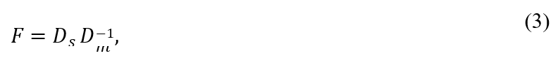
where 𝐷𝑠 = [𝒙1 − 𝒙0, 𝒙2 − 𝒙0, 𝒙3 − 𝒙0], and 𝐷−1m= [𝑿1 − 𝑿0, 𝑿2 − 𝑿0, 𝑿3 − 𝑿0]−1. Note that 𝐷−1m
can be pre-computed from the original undeformed configuration, and 𝐹 is constant within an element. The nonlinear strain tensor is rotation-invariant, thus supports large deformations.
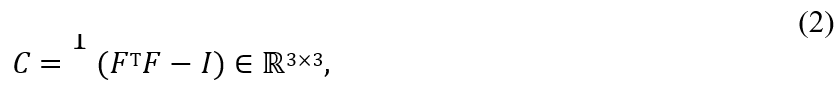
A constraint function can be defined based on the strain tensor, as

With this constraint satisfied, a deformed element can be restored to its initial pose. Since 𝐶 is symmetric, six scalar functions of constraints are derived here, including three stretch constraints with respect to the diagonal components and three shear constraints with respect to the off-diagonal components, written as 𝐶𝑖𝑗(𝒙0, 𝒙1, 𝒙2, 𝒙3) = 0, 𝑖 < 𝑗. For faster convergence of the constraint solver, we use a linearized stretch constraint, 𝐶𝑖𝑖(𝒙0, 𝒙1, 𝒙2, 𝒙3) = √𝑆𝑖𝑖 − 1 = 0, where 𝑆𝑖𝑖 are the diagonal elements of 𝐹T𝐹.
With geometrical constraints, only isotropic deformations can be simulated; and the resulting positional corrections depend on mesh tessellation, which limits the degrees-of-freedom of mesh nodes. For example, the stretch constraint updates nodal positions only along the directions of mesh edges, and the bind constraint also updates positions along a specific direction. In contrast, the strain- based constraints are independent of mesh tessellation and provide the user with more control over the material properties along different directions. In this regard, we have designed an interactive tool to define a frame-field as a reference for defining the anisotropic material properties.
Invertible Volume Constraint
Mathematically, a deformed element can restore its original shape if the strain-based constraints are completely satisfied. However, in the numerical solution, as the strain-based constraints are solved in a Gauss-Seidel-like manner and only by a few iterations, the restoring energy cannot be fully conserved. In our dynamics modelling, we introduce an additional volume constraint for volume conservation, especially in dealing with the large deformations, e.g., deformations caused by fast motion. Given that 𝐽 = det (𝐹) represents the fraction of volume change of an element, 𝐽 = 1 indicates no volume change, we derive a volume constraint as

An advantage of this signed-volume constraint is that, working with our layered constraint solver and the anisotropic frame-field, inverted or even degenerated elements can be restored without special treatments such as the invertible methods in [24,25].
It is also worth to note that the resulting dynamics performance is determined by the constraint functions. We incorporate the strain-based constraints and volume constraint into the dynamic’s integration solver. The strain-based constraints are independent of the mesh grid. The volume constraint is affected by the resolution of the mesh grid but not the geometrical and topological structures.
Layered Constraint Solver for Fast and Stable Convergence
With the primary PBD framework, we can solve a constraint function as follows:
Given a constraint function 𝑓(𝒙) = 0 where 𝒙 is a vector of constrained variables, e.g., position vector 𝒙 = (𝒙0, 𝒙1, 𝒙2, 𝒙3) for a TET element, the position correction vector ∆𝒙 can be obtained by firstly applying a first-order Taylor expansion as

where ∇𝒙𝑓 = 𝜕𝑓/𝜕𝒙 is the gradient of 𝑐 with respect to 𝒙
If we restrict the direction of ∆𝒙 as ∆𝒙 = 𝜆 ∇𝒙𝑓 which conserves the linear and angular momentum, we have ∆𝒙 = (− 𝑐(𝒙) |∇𝒙𝑐|2) ∇𝒙𝑓
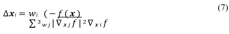
The strength of a certain constraint can be defined by a corresponding stiffness 𝑘, thus the final position correction is taken as 𝑘∆𝒙. This projection process is usually done by a predefined number of iterations in a Gauss-Seidel manner; that is, it solves the constraint element-wisely, and the resulting positional correction of each element immediately affects the following updates. The constraint solver actually propagates the deformations from place to place across the whole TET mesh. It converges to an equilibrium state if an infinite number of iterations are taken.
By decomposing the factors of the above constraint function, it can be seen, for a numerical solution, such a constraint solving scheme requires many iterations to converge; especially for a high-resolution TET mesh, it takes much longer time to propagate a deformation across the mesh. Also, the mechanical behaviors depend on mesh resolution. And finally, the order of constraints affects convergence; that is, if the constraints of elements are solved in a different order, it will produce different deformation behaviors, exhibiting different material stiffness.
To solve these problems, based on the fact that deformations in our rigged TET mesh are propagated from the bone-constrained nodes to the rest of the nodes, we perform a re-ordering of the TET elements into layers according to their distances from the skeleton, such that each bone is surrounded by multi-layers of elements, as illustrated in Figure 2 for two TET meshes. The layers are built from the inner skeleton constrained elements, which are set to be the first layer; and then each successive layer contains the neighbouring elements of the previous layer. The solver will thus encounter the layer-by-layer elements and solve the constraints in a unique way according to the clustered layers. We can achieve a consistent and stable propagation of deformation.
Figure 2. TET elements are re-ordered into different layers (rendered in different colors).
In order to further improve the convergence rate of an iteration, during the first few iterations, we purposely increase the nodal masses of the current layer to consolidate the previous updates after updating nodal positions of each layer (named consolidating iterations here and afterwards) and reset the masses to the original configuration for later iterations. The mass-increasing coefficient can be tuned by the user, which is used as a parameter to control elastic property. In this study, we set it as 10 times of the original mass.
This layered constraint solver requires much less iterations for each animation frame than the conventional PBD scheme. Moreover, it relieves the dependency on different mesh resolutions by increasing the number of consolidating iterations for a higher resolution mesh. These can be validated in our implementation details and results presented in Section 4.
Frame-field for Anisotropic Models
Soft tissues of a character often exhibit anisotropic elastic behaviors, which can be simulated with the strain-based constraints. In order to specify material properties in local frames, a spatially varying frame-field needs to be defined. To generate such a frame-field that specifies a local coordinate-frame for each TET element, we designed an interactive editing tool.
As illustrated in Figure 3, the tool allows the user to input a few NURBS curves on the TET mesh which indicate a fibrous structure of the soft tissues. Local frames can be automatically generated along the curves, forming a sparse distribution of frames. These local frames are generated according to a minimal twist rule called Rotation minimizing frames (RMF). Then, a frame-field is automatically generated by a smooth interpolation of the sparse frames, using a Laplacian smoothing method. Details about the frame-field generation method can be referred to [21].
Figure 3. Local frames defined by the NURBS curves (knots in black and curves in red on the bunny at left), Frame-field generated in the TET mesh (Each node assigned an orthogonal frame, visualized by the red, green and blue vectors respectively).
Each orthogonal frame of the RMFs can be directly represented by a 3 × 3 matrix,

where 𝑚 is the total number of the elements, (𝒓𝑖1, 𝒓𝑖2, 𝒓𝑖3) are the coordinate-vectors of the three axes.
𝑄𝑇 can be considered as a rotation matrix that transforms a vector from the global coordinate system to a local frame.
To incorporate the frame-field control into the dynamics model, the deformation gradient (as in Eq. (3)) of each element should be computed in the local frames as

where 𝑄𝑖 is the local frame matrix in Eq. (8). The inverse matrix in the second term can be pre- computed. Thus, the constraint solver yields a local correction vector ∆𝒙′𝑖, which needs to be transformed back to a global correction vector ∆𝒙𝑖 = 𝑄𝑖∆𝒙′.𝑖
To verify the effectiveness of the proposed methods and their comparative advantages over the previous methods, we implemented a dynamic deformation system. In the experiments, a high-resolution surface mesh is embedded in a coarse tetrahedral mesh for better rendering results, and the surface mesh is deformed by barycentric interpolation of the simulated mesh. A relatively coarse volumetric mesh is useful to boost performance speed. Kinematic motion capture data is obtained from the open Mocap databases [26,27] and [28] in BVH format (refer to [29] for specification). And we use Blender software [30] to edit the skeletal structure in order to match it to a character model.
For more detailed animation results, refer to the accompanying video frames.
Robustness of the rigging scheme: To assess the robustness of the rigging scheme in Section 3.1, we first constrained all the skeleton- intersected elements (as shown in 4a, constrained nodes are rendered as yellow points), which turned out to produce undesirable artifact of outliers, as shown in Figure 4b and Figure 4c. If the nodes of a constrained element are attached to different bones, outliers are produced due to the volume constraint. We referenced to the previous work [19,20] which requires an additional bind constraint to maintain the distance between a node and a related bone. While such a constraint can suppress the outliers, it is computationally expansive, especially in high-resolution mesh models.
Figure 4. Constrained elements by the skeleton. In (a), all the elements intersected by the skeleton are constrained, producing outliers shown in (b) and (c). In (d), bone-shared elements are excluded, and correct deformations are produced shown in (e) and (f).
We adjusted our rigging scheme by revisiting the intersecting TET elements. Those tetrahedral nodes around the joints and intersected by more than one bone are released from the constraint (note the elimination of the yellow points in Figure 4d). The following experiments show the corrected deformation behaviors around all the joints in Figure 4e and Figure 4f. This correction is largely credited to our layered constraint solver which compensates the constraints of the eliminated intersecting element nodes with their neighbourhood in the inner layer. This strategy makes the time-consuming bind constraint in dynamic deformation computation unnecessary.
Comparisons of skinning methods: To verify the advantages of the strain-based constraints and volume constraint introduced in Section 2.2-4, we first compare our method with the conventional LBS and DQS in different scenarios. As shown in Figure 5a, the LBS suffers from a widely known candy-wrapper artifact when performing a twisting motion. Whereas LBS produces a better deformation (Figure 5c), DQS suffers from a bugling- joint artifact with a bending motion (Figure 5d) - a textured-cylinder model is used to provide a better visual reference for the comparisons. None of these geometrically based skinning methods can produce satisfactory deformations suitable for all scenarios. Since our skinning method works with the physically based constraints, realistic deformations can be produced without suffering from these artifacts. Volume is well preserved, as shown in Figure 5b and Figure 5e. There is no need for a weight- painting refinement process as is used in the previous methods. Moreover, secondary motions (e.g., contractile muscle in the upper arm) are naturally generated.
Figure 5. Comparison of dynamics models: LBS, DQS and our method.
Comparisons of unordered and layered constraint solvers:
We now compare the results of unordered constraint solver and our layered constraint solver introduced in Section 3.5. As shown Figure 6, a jumping leg model (with 24387 TET elements) is simulated, where all the three rows are simulated by the same constraint coefficients and time-step size. The unordered solver converges slowly, as shown in Figure 6a and 6b. 10 iterations are far from convergence in Figure 6a, and 50 iterations are needed to obtain satisfactory behaviors as shown in Figure 6b. In contrast, the re-ordered layered constraint solver takes only 10 iterations (with the first 6 as consolidating iterations) to achieve the same convergence as in the 50 iterations of the unordered solver, as shown in Figure 6c. This validates the fast convergence rate of the proposed ordered solving scheme, which greatly reduces computational cost for solving the constraints.
Figure 6. Comparison of the unordered solver and our layered constraint solver.
To test the consistency of the dynamic’s models, we varied the resolution of the TET mesh. As expected, with the unordered solver, convergence rates for meshes with different resolutions differ a lot. In Figure 7, a lower-resolution leg model (with 3452 TET elements) is simulated with the same constraint coefficients and time-step size as in Figure 6. The unordered solver with 10 iterations converges much faster with the low-resolution mesh in Figure 7a, compared to its high-resolution counterpart in Figure 6a. This poses the difficulty for deformation control of meshes with different resolutions, due to large deformation behaviour differences among them.
Figure 7. Comparison of the unordered solver and our layered constraint solver in a low-resolution mesh.
Our reordered layered constraint solver largely alleviates this problem. As shown in Figure 7b and 7c, with the same setting with Figure 6c, the same 10 iterations achieve the same deformation of its high-resolution counterpart. A further flexibility of the material property of stiffness can be obtained by adjusting the number of consolidating iterations (6 in Figure 7b and 2 in Figure 7c). Therefore, deformation control can be done at similar performance level by using the reordered solver.
Comparison of isotropic and anisotropic deformations: To verify the effectiveness of the frame-filed incorporated into an anisotropic model discussed in Section 3.6, we present the deformations of models with isotropic and anisotropic materials respectively in Figure 8.
Figure 8. Comparison of isotropic and anisotropic deformations (The surface model is obtained from Blender open movie project [31]. The accompanying video demo can better reveal the details).
We again reference to the representative work [19,20] on the PBD framework. As they use geometrical constraints, it is impossible to define the dynamics model of anisotropic materials, in particular, the model cannot accommodate the anisotropic frame-field in the TET mesh with an irregular grid. Without a reference frame-field, we can only define isotropic materials: the strain-based constraints are solved in a single global frame, and there are only two strain-based coefficients, i.e., stretch stiffness and shear stiffness. Isotropic deformations of the bunny model are shown in Figure 8a.
With the frame-field as shown in Figure 3, where each frame is represented by three axes (𝒓, 𝒈, 𝒃) rendered in red, green, and blue colors respectively, totally six constraint coefficients can be defined: three stretch coefficients and three shear coefficients along three directions of each local frame for each TET element. We adjust the six parameters to define an anisotropic material. The anisotropic setting exhibits much more expressive deformations, such as the wrinkles formed at its belly and more flexible behaviors at the ears, as shown in Figure 8b.
Executive performance analysis: To assess the computational performance and demonstrate the effectiveness and robustness of our dynamics modelling system, we conducted more experiments with large ranges of motions, secondary motions, and anisotropic material properties. Details can better be revealed in the accompany video, and Figure 9 and Figure 10 are the screenshots.
Figure 9. Skeleton-driven animation of a fatman model (Surface model courtesy of Kim [13]).
Figure 10. Skeleton-driven animation of a kicking man model.
An un-optimized implementation of the algorithms was written in C++. All the examples are executed on a desktop with Intel Core CPUs (i7-4770 @3.40GHz). The time-step size of the constraint solver is made consistent with the framerate of the Mocap data (120Hz with the male model, and others with 30Hz or 25Hz). Statistics and executive performance of the examples are given in Table 2. It shows that the frame-field incorporated dynamics model costs only a small fraction of time more than its counterpart without a frame-field, mainly for the local-frame computations. All the deformations are done within 10 iterations for the constraint solver, thanks to the layered solving scheme. Therefore, real-time performance can be achieved, making the modelling system viable for various applications.
Table 2. Executive performance on different animation models.
Notes on Non-Decoupled Shear Constraint
For purely elastic models [22], a decoupled shear constraint 𝐶𝑖𝑗 (𝒙0, 𝒙1, 𝒙2, 𝒙3) = √𝑆𝑖𝑗 |𝑆𝑖𝑗|= 0, 𝑖 < 𝑗 can also be used, which decouples shear from stretch and penalizes only the angular deformation. However, this decoupled shear constraint is nonlinear along the projection direction. It causes overshooting problem that leads to failure in our dynamics modelling experiments with the anisotropic material property, when large bending angles occur at the joints.
To deal with this problem, a non-decoupled shear constraint was explored in our system, which can affect the stretch stiffness of an element. Combining it with the volume constraint, however, might result in an over-constrained system, producing jittering artifacts. We analyzed such cases and proposed a few techniques to minimize the unwanted effects in deformation, for example, by decreasing the stiffness of the volume constraint.
We have also noticed the problem in the conventional PBD framework that material stiffness depends on not only the constraint coefficients but also the time-step size in the constraint solver. We propose a constant time-step size which is according to and consistent with the framerate of the skeleton motion.
We have presented a strain-constrained body mesh deformation system based on skeleton-driven dynamics modelling. Strain-based constraints are incorporated into the PBD framework, which has shown great improvement on physically plausible deformation compared with those using the geometrically based skinning techniques such as LBS and DQS. It turns out to be effective and efficient for animating characters. Natural secondary motion of soft tissues can be produced, and anisotropic deformation behaviors can be intuitively controlled by using a designed frame-field. Stretch and shear coefficients can be easily tuned to change material stiffness along different directions. The constraint solver converges fast with a re-ordered layered solving scheme. Stable and consistent execution performance can be achieved.
Compared with the most related work: (1) our method avoids the LBS computation, and no weight function needs to be defined; instead, a fast rigging is performance to update the constrained nodes; (2) In our method, strain-based constraints instead of geometrical constraints are exploited, which makes the definition of material properties independent of mesh grid, and anisotropic materials can be defined; no bind constraint is needed to compute the rest distance between a node and its projection on the skeleton. (3) With the layered constraint solving scheme, our solver converges much faster and is more predictable in deformation.
There is still room for improvement in the future. First, volume can be well preserved for each element; however, without dealing with self-contact, self-penetration artifacts can occur. In the future, self-collision constraint should be exploited in order to obtain more accurate deformation behaviors. Secondly, there is only a one-way interaction between the skeleton and the simulated mesh in the current system; that is, motion of the mesh is driven by the skeleton. A two-way coupling approach can be incorporated into the system. The motion of the soft tissues can also affect the movements of the pre-defined motion of skeleton. This would be helpful to apply a same Mocap data to characters of different sizes and weights and re-generate different locomotion that respects their different characteristics. And finally, better tetrahedralization algorithm should be developed to generate TET mesh with qualified layers of elements, which would improve the performance of the layered constraint solver.
Implementation of the proposed algorithms is based on the open-source Vega FEM library [32]. This work is supported by the grants, MOE AcRF RG93/20, Ministry of Education, Singapore.
- Magnenat-Thalmann N, Laperrire R, Thalmann D (1988) Joint- dependent local deformations for hand animation and object grasping. In Proceedings on Graphics interface’88, Citeseer.
- Kavan L, Collins S, Žára J, O'Sullivan C (2007) Skinning with dual quaternions. Proceedings of the 2007 symposium on Interactive 3D graphics and games, ACM.
- Kavan L, Collins S, Žára J, O'Sullivan C (2008) Geometric skinning with approximate dual quaternion blending. ACM Transactions on Graphics (TOG) 27: 105.
- Kim YB, Han JH (2014) Bulging‐free dual quaternion skinning. Comp Anim Virtual Worlds 25: 321-329.
- Jacobson A, Deng Z, Kavan L, Lewis JP (2014) Skinning: Real-time shape deformation. ACM SIGGRAPH Course.
- Terzopoulos D, Platt J, Barr A, Fleischer K (1987) Elastically deformable models. SIGGRAPH Comput Graph 21: 205-214.
- Nealen A, Mueller M, Keiser R, Boxerman E, Carlson M (2006) Physically Based Deformable Models in Computer Graphics. Computer Graphics Forum 25: 809-836.
- Sifakis E, Barbic J (2012) FEM simulation of 3D deformable solids: a practitioner's guide to theory, discretization and model reduction. ACM SIGGRAPH, ACM.
- Steve C, Burkhart M, Curless B, Duchamp T, Popović Z (2007) Physically based rigging for deformable characters. Graphical Models 69: 71-87.
- Steve C, Burkhart M, Curless B, Duchamp T, Popović Z (2002) Interactive skeleton-driven dynamic deformations. ACM Trans Graph 21: 586-593.
- Teran J, Sifakis E, Irving G, Fedkiw R (2005) Robust quasistatic finite elements and flesh simulation. Proceedings of the 2005 ACM SIGGRAPH/Eurographics symposium on Computer animation. Los Angeles, California.
- Gilles B, Bousquet G, Faure F, Pai DK (2011) Frame- based elastic models. ACM Trans Graph 30: 1-12.
- Kim J, Pollard NS (2011) Fast simulation of skeleton-driven deformable body characters. ACM Trans Graph 30: 1-19.
- Kim T, James DL (2011) Physics-based character skinning using multi- domain subspace deformations. IEEE Trans Vis Comput Graph 18: 1228-1240. [Crossref]
- Müller M, Heidelberger B, Hennix M, Ratcliff J (2007) Position based dynamics. J Vis Comun Image Represent 18: 109-118.
- Bender J, Koschier D, Charrier P, Weber D (2014) Position-based simulation of continuous materials. Computers & Graphics 44: 1-10.
- Deul C, Bender J (2013) Physically-Based Character Skinning. Virtual Reality Interactions and Physical Simulations 13: 25-34.
- Müller M, Chentanez N (2011) Solid simulation with oriented particles. ACM Transactions on Graphics 30: 92.
- Rumman NA, Fratarcangeli M (2014) Position based skinning of skeleton- driven deformable characters. Proceedings of the 30th Spring Conference on Computer Graphics, ACM.
- Rumman NA, Fratarcangeli M (2015) Position‐Based Skinning for Soft Articulated Characters. Computer Graphics Forum.
- Cai J, Lin F, Lee YT, Qian K, Seah HS (2016) Modeling and dynamics simulation for deformable objects of orthotropic materials. The Visual Computer 33: 1307-1318.
- Müller M, Chentanez N, Kim T-Y, Macklin M (2014) Strain Based Dynamics. Eurographics/ACM SIGGRAPH Symposium on Computer Animation.
- Bower, Allan F (2009) Applied mechanics of solids, CRC press.
- Irving G, Teran J, Fedkiw R (2006) Tetrahedral and hexahedral invertible finite elements. Graph Models 68: 66-89.
- Stomakhin A, Howes R, Schroeder C, Teran JM (2012) Energetically Consistent Invertible Elasticity. Eurographics/ACM SIGGRAPH Symposium on Computer Animation.
- CMU Graphics Lab Motion Capture Database. (http://mocap.cs.cmu.edu/).
- Huang J, Shi X, Liu X, Zhou K, Guo B, et al. (2006) Geometrically based potential energy for simulating deformable objects. The Visual Computer 22: 740-748.
- NUS Mocap Database, http://animation.comp.nus.edu.sg/nusmocap.html
- Biovision BVH File Specifications page, http://www.character- studio.net/bvh_file_specification.html.
- Blender-free and open source 3D creation suite. https://www.blender.org.
- Blender (2008) Big Buck Bunny. https://peach.blender.org/
- Barbič J, Sin FS, Schroeder D (2012) Vega FEM Library: http://www.jernejbarbic.com/vega.