Electroplating or electrodeposition is a process carried out in an electrochemical cell where a current is used to form a coating on a metal surface. Developing and optimizing conditions for electroplating is time consuming and modeling and simulation could be used to optimize the electrodeposition process. Electrolyte current density and conductivity are important parameters for an electrodeposition system as they dictate the overall efficiency of flow of ions in the electrolyte system and thus optimization of these parameters is necessary. In this manuscript we report the development of a mathematical model to predict the electrodeposition of copper on cobalt chrome alloy in an electrochemical cell with copper and cobalt chrome alloy as the electrodes and copper sulfate as the electrolyte. The developed model was validated using experiments. The coating thickness of the samples was characterized using scanning electron microscope (SEM) and a thickness gage. At 30 min the model predicted the copper thickness to be 11.7 µm while experimentally the coating thickness was found to be 9.445+/-1.79 (mean +/- SD) using SEM and 12.375+/-1.36 (mean +/- SD) using thickness gauge. When predicting effect of current density the model accurately predicts general trends however the model seems to vary from experimental values in regions where there is significant effect of the electrochemical double layer that the model does not account for. The model accurately predicts the trend of effect of electrolyte conductivity on coating formation. The model can thus be used as a starting point to predict effect of process parameters on electrodeposition thickness
multiphysics modeling, electrodeposition, electroplating, Co-Cr alloy
Simulation using mathematical modeling is a tool that is used to predict, evaluate or optimize the performance of a proposed / current system under study over time [1,2]. Simulation is performed under specific input conditions and output of the model is compared with that of the actual system [3]. Physical processes could be modeled to minimize experimental trials necessary for optimization of the physical process [4]. Simulation modeling helps designers and engineers to understand the ways and conditions, in which a part could fail, the loads it can withstand and helps to avoid recurring usage of physical prototypes to analyze designs for new and existing parts [5]. There are various types of simulation modeling such as stochastic [6], dynamic [7] and Multiphysics modelling [8]. A stochastic model is performed from a source of randomness as it is based on certain assumptions of the system under study [9]. Statistical modeling is a stochastic model [10]. Examples of this type of modeling are linear regression [11], multiple regression [12], etc. Monte-Carlo method is a type of stochastic modelling [13]. Dynamic modelling [14] represents time aspect of a system. Simulation modeling used for optimizing material handling in a plant would be an example under this category [15]. Multiphysics modeling incorporates principle of physics, chemistry biology and engineering in a mathematical statement that describes the phenomena or system under consideration [16].
Electroplating or electrodeposition is a process carried out in an electrochemical cell where a current is used to form a coating on a metal [17]. In the electrochemical cell the metal to be coated is the cathode and the anode can be one of the two: sacrificial anode (dissolvable anode) or permanent anode (inert anode) [18]. Electrolyte in the electrochemical cell acts as a medium for the movement of electrons and forms the electric circuit between the electrodes [19]. Oxidation occurs at the anode while reduction reaction occurs at the cathode resulting in electrodeposition [20]. Electroplating is used for various applications including corrosion protection [20]. For example, electroplating of Palladium is used to manufacture catalytic converters because it has the ability to absorb excess hydrogen. Fasteners are electro-plated to have a better corrosive resistance [21]. Majority of the electrical parts and components are used after electro-deposition process. Silver electroplating has been used on copper or brass to enhance its conductivity and also used in silicon solar cells to increase its operating efficiency by 0.4% [22]. Nickel plating, tin plating and various alloys are used for corrosion protection on nuts, bolts, housings, brackets, other metal parts and components [23]. Though expensive, gold electroplating provides not only corrosion, but also tarnish protection [24].
Developing and optimizing conditions for electroplating is time consuming and modeling and simulation could be used to optimize the electrodeposition process. Various examples exist in the literature that demonstrates the benefits of modeling of electrodeposition to predict plating outcomes [25-27]. For example Obaid et al., modeled the electroplating of hexavalent chromium to optimize the electrode spacing and anode height to obtain uniform thickness of the coating [28]. Loss of coating uniformity was observed when the electrode spacing decreased while greater electrode distance increased the uniformity of the formed coating [28]. The simulation results proved that an ideal electrode separation distance was necessary to obtain a uniform coating. It was also proved that, larger size of anode as compared to cathode resulted in a non-uniform coating [28]. Hughes et al., demonstrated that the electrode kinetics played an important role in the electrodeposition process [29]. Electrode kinetics defined the deposition process using the rate determining step and current distributions. Their simulation results proved that variables like surface electrode potential and the ion concentration in the electrolyte also influenced the kinetics associated with the deposition process [29].
Optimization of electrodeposition of new systems would require optimization of process conditions relevant to that system. This would require significant changes to a model or developing a new model specific to that system. Electrolyte current density and conductivity are important parameters for an electrodeposition system as they dictate the overall efficiency of flow of ions in the electrolyte system and thus optimization of these parameters is necessary. In this manuscript we report the development of a mathematical model to predict the electro deposition of copper on cobalt chrome alloy in an electrochemical cell with copper and cobalt chrome alloy as the electrodes and copper sulfate as the electrolyte.
Governing equations
A mathematical model was developed to predict the electrodeposition of copper on cobalt chrome alloy and to evaluate the effect of electrolyte current density and conductivity on electroplating thickness. Electroplating occurs due to mass transport in the solution as a result of migration in electric field, diffusion in concentration gradient and convection in a flow field [30]. The transport equation which was applied in the diffusion layer was based on the flux equation of the ionic species in the solution. The general mass balance equation is given below
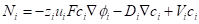
Where Ni- molar flux, Zi - charge number, Ui - mobility, F – Faradays constant, Ci - concentration, Di – Diffusivity, ∅ - potential in the electrolyte, V - velocity
The flux equations explaining the behavior of electrochemical systems are related to the Second Law of Thermodynamics [31]. Consider two neighboring volume elements V' and V'' of a solution that have same temperature and pressure but different electrochemical potentials of their constituents. The difference between the electrochemical potential of species i,  and , in these volume elements implies that this species tends to move from one volume element to the other as there is no distribution equilibrium. This motion of species i from one volume element to its neighbor is generically called transport of species i. As the transport of the different species in solution takes place under thermal and mechanical equilibrium, the change in internal energy U of these two volume elements is
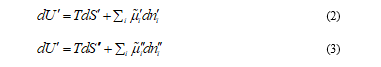
Where T is the thermodynamic temperature, S is the entropy and ni the number of moles of species i. Considering the exchange of matter between V' and V'', which takes place without energy exchange with their surroundings, it is satisfied that

Each individual term of the sum is positive when the transport of species i is not coupled to transport of other species. In this case,  is determined only by
  and species i moves towards the region in which its electrochemical potential is lower, that is,
 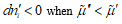 and vice versa. For example, this takes place in the case of ionic species in diluted solutions. When the transport of different species is coupled, one or more terms in the sum could be negative, but the sum is always positive.
The transport of the species i is described in terms of either its velocity  or its flux density
  . If the area of the surface between the two volume elements is dA and its orientation is given by the unit vector
 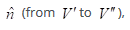 the number of moles of species i crossing the surface in a time dt is
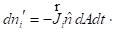
When the difference between is not very large, it can be assumed that the rate of change of the amount of species i,
  is proportional to the difference
  or to the gradient of this potential normal to the surface,
  . The velocity of species i in linear approximation is expressed as

Where ui is its mobility
Flux density takes the form

Where R is the universal gas constant and the Einstein relation between mobility and diffusion coefficient, Di=ui RT, has been used.
At constant temperature and pressure, the gradient  is caused by the changes in composition and electrical potential ø so that
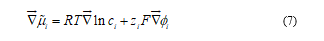
Where F is the Faraday constant and zi the charge number of species i. Substituting Equation (7) in Equation (6), the Nernst-Planck flux equation
is obtained, where f denotes the ratio F/RT. The terms in the righthand side of this equation represent the transport mechanisms of diffusion and migration, respectively. Diffusion is a consequence of the random thermal motion of the particles which makes the concentration of all species uniform. Migration causes the influence of the electric field,  , on the random motion of the charged particles, and Equation (8) shows that the particles a component of their velocity along the direction of the electric field as a result of this influence.
Flux of species i due to bulk flow in a moving fluid in X-direction,

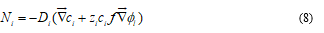
Therefore, the flux expression for each species i can be written as

Where the ionic mobility ui, is assumed to be related to the diffusion coefficient Di by the Nernst-Einstein equation [32]
The material balance equation for each ionic species at every point within the diffusion layer is as follows
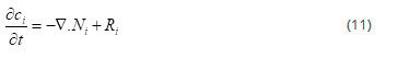
Where Ri is the production rate of species i due to homogeneous chemical reactions.
Under the assumption, variations in composition are negligible in the electrolyte and migration of ions gives the net contribution to current in the electrolyte equation.
The concentration gradients in the above equations are neglected in the Secondary Current deposition interface and the current density is obtained from Ohm’s law

Where σl denotes the electrolyte conductivity.
Since the electrolyte composition is assumed to be constant, the material balances are unsolved for the Secondary current distribution,
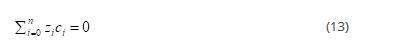
The electroneutrality condition is given by the following expression:
Electrode kinetics
Electrodeposition is a combination of oxidation and reduction reactions occurring at the electrodes making the electrode kinetics very significant for the modeling of electrodeposition.
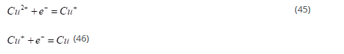
Consider the reaction given below:

Kf and Kb are the rate constants of the forward and backward reactions respectively.
Reaction rates: The reaction rate, also known as rate of reaction or speed of reaction, for a reactant or product in a particular reaction is defined as how fast or slow a reaction occurs.
Equilibrium: Equilibrium is point at which the net reaction rate is zero. From the above equations, we can obtain the equilibrium concentration ratio as follows
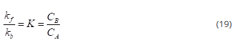
Where K is the equilibrium constant (K)
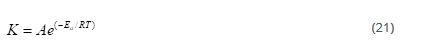
Rate constant varies with temperature, generally it increases with T. The rate constant (K) and temperature are related by:
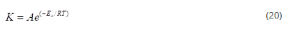
Where, Ea=activation energy, R=gas constant and A=pre exponential factor
Activation energy: Activation energy [33] is the barrier that has to be overcome by the reactants before they are converted to product. More energy is required by the reactants when there is a larger barrier for the activation energy.
Exponent term  is a probabilistic feature of the energy barrier component which has to crossed.
Pre exponential factor A, also known as frequency factor, gives a number of times the attempt was made to overcome the energy barrier consider the electrode reaction:

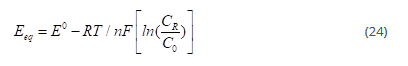
Where kf and kb are the forward and backward reaction rate constants respectively. This is a general redox reaction, where O represents oxidized state and R represents reduced state. For this reaction, the equilibrium state is governed by the Nernst equation, which relates the equilibrium potential of the electrode (Eeq) to the concentration of the reactants and products (O and R)

Overvoltage: A given current will require a penalty that should be paid in terms of electrode potential-penalty called overvoltage [34] due to irreversibility.
E_eq is the expected electrode potential and E is the electrode potential

Where a and b are constants and I is the current density. This is the Tafel equation.
Kinetics of electrode reactions:
Rates of forward and backward reaction

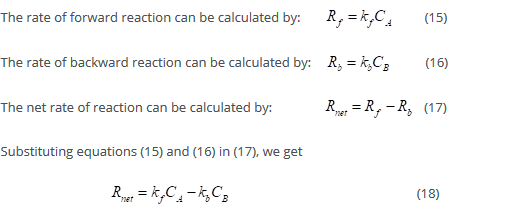
For the above reaction, the rate of the forward reaction is given by:

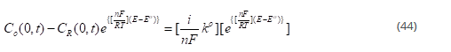
Where Co(0,t) is the surface concentration of O.
Rate of the backward reaction is given by:

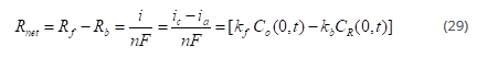
Reaction rate and current are correlated. Reduction occurs at the cathode and oxidation at the anode.
Net reaction rate:
The net reaction rate or net current is given by
Potential dependence of kf and kb
Both kf and kb are potential dependent functions
The forward reaction, which is a reduction, is an electron accepting process. The rate of reaction increases when the electrode potential reaches higher negative because the electrode loses electrons more easily. The opposite happens in the backward reaction, i.e., oxidation reaction.
At equilibrium:
The electrode potential and oxidation and reduction concentrations make net reaction rate zero. Thus:
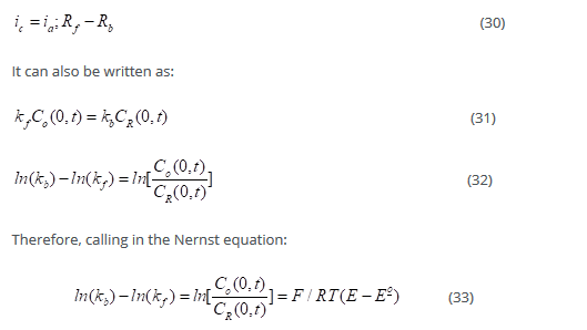
Upon differentiating the above equation with respect to E, we get:
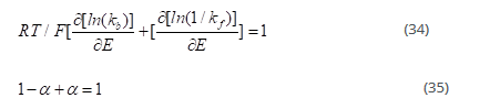
The terms on the left hand side of the reaction sum up to 1 and called symmetry factors (for one electron transfer in the reaction).
Reductive and oxidative symmetry factors
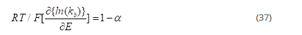
The reductive symmetry factor is associated with the forward reaction which is represented by α
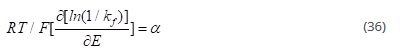
The oxidative symmetry factor therefore becomes (1-α)
The term α is the measure of the symmetry of energy barrier. If the change in the potential is same on both sides of the barrier, then α=0.5=1- α. Any asymmetry in the change causes fractional values of α.
Standard rate constants:
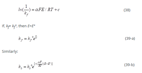
kf° and kb° are termed as standard rate constants
If the concentrations of oxidation and reductions are same, and the potential is maintained at Eº to cause any current flow:
From above equation, kf° = kb°
The larger the value of Kº, the faster is the equilibrium. Reactions with small standard rate constants are slow. The standard rate constant is large for simple redox couples
The Butler-Volmer theory

Where n is the number of electrons transferred. This is the Butler –Volmer [35] formulation of electrode kinetics. There are two components, of current i.e., anodic and cathodic, and it is exponentially dependent on potential. The net reaction rate is given by:
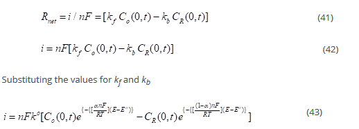
This formulation is called the Butler –Volmer formulation of electrode kinetics
At Equilibrium:
At equilibrium, i=0
2.3. Thickness of deposition
The deposition process is assumed to take place through the following simplified mechanism:
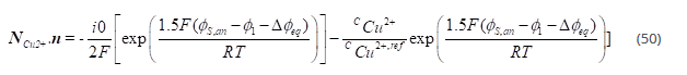
The first step is rate determining step (RDS), and the second step is assumed to be at equilibrium, which gives the following relation for the local current density as a function of potential and copper concentration:
where n denotes the over potential defined as

where ∅(s,0) denotes the electronic potential of the respective electrode.
Equation at the cathode is given by:
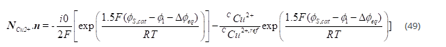
where n denotes the normal vector to the boundary.
Equation at the anode is
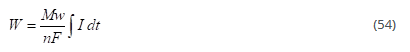
The amount of deposition is understood by the Faraday’s laws of electrolysis [36] which states that the amount of a material deposited on an electrode is proportional to the amount of electricity used. For reduction of one mole of a given metal ion (charge of n+), n moles of electrons are used for reduction. The total cathodic charge for the coating, Q(C), is the product of the number of gram moles of the metal coated, m, and the number of electrons required for the reduction reaction, n, Avogadro’s number, Na (number of atoms in a molecule), and the electrical charge per electron, Qe(C). Thus, charge required to reduce m moles of metal is given by

The product of Avogadro’s number, Na (the number of atoms in a mole), and the electrical charge per electron, Qe(C) gives the Faraday constant, F. The number of moles of the metal reduced by charge Q is:

The total charge used in the deposition can be calculated by the product of the current, I (A), and the time of deposition, t (sec), where the deposition current is constant. When current varies with time during the deposition process, Q can be calculated by,

The weight of the deposit, W(g), can be calculated by product of the number of moles of metal reduced and atomic weight, Mw, of the deposited metal is given by:
The thickness of the deposition, d (cm), can be solved by:
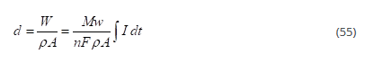
Where ⍴ is the density of the metal (g = cm3) and A is the area of deposition (cm2).
Boundary conditions
All boundaries (B1 and B4) were insulating:
Initial conditions
The initial conditions of the electrolyte were:
Figure 1 shows the schematic representation of electrodposition and the corresponding model geometry for simutaltion of the electrodeposition process. Finite element methods were used to discretize the multiphysics governing equations. A finite element solver software COMSOL was used to simulate and predict plating thickness under varied process conditions. The model was set as a two diemnsional (2D) time dependent model (Figure 1). The deposition at cathode and the dissolving of the anode was set to take place at 100% current yield. During the electroplating process, changes in the electrolytic density of the electrochemical cell occurs which would result in the change in the density at anode and cathode. These changes could induced free convection in the cell, however based on our assumption that the variation in composition is small, the free convection component was neglected.
The process was assumed to be time dependent as the boundary of the cathode was moving as the deposition of the metal was taking place. The model is governed by mass conservation for the copper ions Cu2+ and sulphate SO4-2 and the electroneutrality condition. The upper boundary represented anode, and cathode was placed at the bottom. The vertical walls were assumed to be insulated (Figure 1).
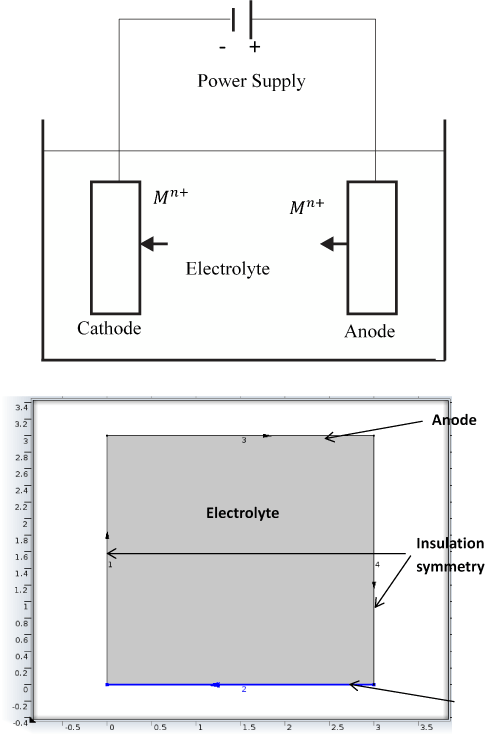
Figure 1. Schematic Depiction of Electrodeposition (top) and Corresponding Model Geometry for Simulation of the Electrodeposition Process (bottom).
The developed mathematical model was validated experimentally. The electroplating of Copper on Cobalt-Chrome was conducted in a electrolytic cell. The electrolytic solution was prepared with 100 gms. of CuSO4 in 100 ml of distilled water and 7 ml of 1N of H2SO4. The solution was kept on the stirrer to mix homogenously. A cobalt chrome strip of 14 cm × 14 cm was taken and an immersion area 1.4 cm × 1.4 cm cm was used and copper strip of 14 cm × 14 cm was taken and an immersion area 1cm × 1cm was used. The copper strip was connected to the anode and the cobalt chrome was connected to the cathode were immersed in the electrolyte and then current was passed. Electroplating was conducted under varying electrolyte conductivities such as; 4.23 S/m2,1.9 S/m2, 0.93 S/m2 and 0.54 S/m2 and varying current densities such as; 2.52 × 10²(A/m2), 3.57 × 10²(A/m2) and 6.12 × 10²(A/m2). Post deposition the samples were air dried and characterized for coating thickness. The samples were characterized with Scanning electron microscope (SEM) and a thickness gauge. For thickness analysis using SEM across sectional view of the coated sample was taken and the thickness of the coating determined. Four replicates were carried out and the coating thickness values were reported as mean +/- standard deviation (SD). An analysis of variance, ANNOVA (two way/one way) was used to determine statistical significant differences at the 95% confidence level.
Figure 2 shows the thickness change of the electrodeposited copper on cobalt chrome alloy versus time as predicted by the developed mathematical model. From the simulated results (Figure 2) we see that for the first 500 sec the coating hasn’t started, as the time goes by we see a steady coating of Cu on Co-Cr. At the end of 3000 sec we see the predicted coating thickness on Co-Cr to be 0.019 mm. To validate the model an electrodeposition experiment was carried out with same parameters as the model prediction for duration of 30min (1800 secs). Electrolyte test parameters for this experiments included an electrolyte conductivity of 4.23 S/m2, current density of 3.57 × 10²(A/m2) and a 1.4 cm × 1.4 cm area of contact. Four replicates were carried out to evaluate the variance of test results. The samples were characterized with Scanning electron microscope (SEM) and a thickness gauge to measure the thickness of the coatings formed.
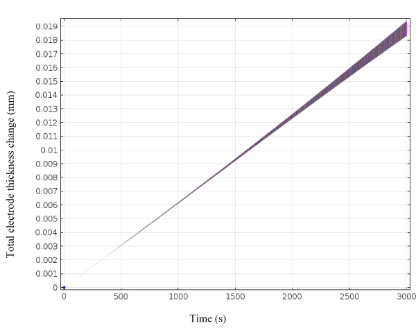
Figure 2. Electrodeposited copper coating thickness change on cathode as a function of time.
Figure 3 shows a representative SEM image used for calculation of the coating thickness while the thickness gauge was directly used on the sample to measure the thickness. For each sample measurement readings were taken at four different points and the average reported. Figure 4 shows the comparison of modeled (simulated) thickness and experimentally obtained thickness values.
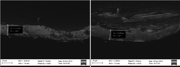
Figure 3. Representative SEM images that were used for evaluating elecrodeposited copper coating thickness.
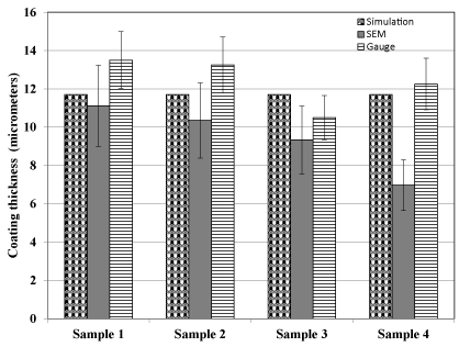
Figure 4. Comparison of modeled and experimentally determined electrodeposited copper coating thickness values.
From Figure 4 and Table 1, it can be seen that at 30 min the model predicted the copper thickness to be 11.7 µm (0.0117 mm) while experimentally the average coating thickness was found to be 9.445+/-1.79 (mean +/- SD) using SEM and 12.375+/-1.36 (mean +/- SD) using thickness gauge. Figure 4 shows that there was lot of variation of thickness values when using SEM as compared to the thickness gauge. It can be seen (Figure 4) that the thickness gauge measurement values (12.375+/-1.36) were found to be closer to the predicted values (11.7) as compared to that of SEM thickness values (9.445+/-1.79). This variation could be attributed to the challenges associated with using the SEM for measuring coating thickness. In SEM a precise cross sectional view was required to measure the thickness accurately. Deviation from an accurate cross sectional view (90O) could result in variation of thickness values. Also if the layer was not uniform it could cause variation in the thickness values measured. Thickness gauge measurements were relatively consistent in its measurements. However the relative accuracy of the predicted and experimental values validates our model. This demonstrates the preliminary applicability of the model in predicting electro deposition of copper on cobalt chrome substrate.
Table 1. Experimental validation of mathematical model.
|
|
Thickness (micrometer) at 30 min (1800 secs) |
|
Current |
Simulation |
SEM
(Mean +/-SE) |
Gauge
(Mean +/-SE) |
Sample 1 |
0.07 A |
11.7 |
11.12+/-0.4 |
13.5+/-0.29 |
Sample 2 |
0.07 A |
11.7 |
10.35+/-0.53 |
13.25+/-0.48 |
Sample 3 |
0.07 A |
11.7 |
9.33+/-0.3 |
10.5+/-1.85 |
Sample 4 |
0.07 A |
11.7 |
6.98+/-0.13 |
12.25+/-0.85 |
Average |
|
|
9.445+/-1.79 |
12.375+/-1.36 |
Effect of current density on coating thickness
To evaluate the effect of current density on coating thickness the model was used to simulate and predict the electroplating thickness at three different current densities. This experiment was conducted with different current densities at an electrolyte conductivity of 4.23 S/m2 on 1.4 cm × 1.4 cm area of contact. The different current densities used were 2.52 × 10²(A/m2), 3.57 × 10²(A/m2) and 6.12 × 10²(A/m2). The experimental and predicted values are shown in Figure 5 for duration of 46 minutes.
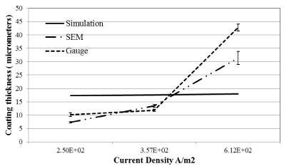
Figure 5. Simulated and experimental coating thickness at varying current densities at 46 minutes.
From figure 5 and Table 2 we can see that the model predicted a coating thickness of 17.3, 17.6 and 18 micrometers at current density of 2.52 × 10²(A/m2), 3.57 × 10²(A/m2) and 6.12 × 10²(A/m2) respectively. The model thus predicts negligible differences with changes in current density. The experimental value of the coating thickness conducted under same conditions showed significant differences when compared to the simulated values. Figure 5 showed experimental values to be lower than simulated conditions at lower current densities 2.50 × 10²(A/m2) and 3.75 × 10²(A/m2) while experimental values were higher than simulated values at higher current density of 6.12 × 10²(A/m2). This can be explained by the formation of an electrochemical double layer surrounding the electrodes which plays a critical role in the diffusion of ions from and towards the electrodes. The phenomenon of electrochemical double layer and its effect on diffusion of ions has been well documented in the literature [37-39]. At lower current density there will be a higher resistance from the double layer resulting in fewer ions going through the double layer resulting in lower coating values. While at higher current density the ions overcome the resistance of the double layer which results in higher coating thickness. The developed simulated model currently does not account for the double layer formation and its effect on coating thickness. This is something that will be needed to be incorporated to simulate more accurate predictions over a wide range on current densities. Comparing SEM and gauge thickness values we see similar higher difference with larger coating thickness as compared to lower thickness due to larger variances SEM measurements as discussed previously.
Table 2. Effect of current density on coating thickness.
Thickness (micrometer) |
Current Density - 2.50 E+02 (A/m2) |
Time (min) |
Simulation |
SEM
(Mean +/-SE) |
Gauge
(Mean +/-SE) |
18 |
7 |
2.33+/-0.09 |
5+/-0.41 |
25 |
9.5 |
4.65+/-0.31 |
6.75+/-0.48 |
40 |
14.3 |
6.9416+/-0.09 |
11.5+/-1.19 |
46 |
17.3 |
7.3912+/-0.23 |
10.2+/-0.73 |
Current Density - 3.57 E+02 (A/m2) |
Time (min) |
Simulation |
SEM
(Mean +/-SE) |
Gauge
(Mean +/-SE) |
46 |
17.6 |
13.455+/-0.47 |
11.8+/-0.37 |
Current Density - 6.12 E+02 (A/m2) |
Time (min) |
Simulation |
SEM
(Mean +/-SE) |
Gauge
(Mean +/-SE) |
18 |
7 |
8.68+/-0.9 |
4.4+/-0.81 |
25 |
9.8 |
8.964+/-0.34 |
8+/-0.45 |
40 |
15.2 |
23.49+/-1.27 |
34+/-1.87 |
46 |
18 |
31.35+/-2.43 |
42.75+/-1.25 |
Figure 6 and Figure 7 shows the coating thickness vs time for current density of 6.12 × 10²(A/m2) and 2.50 × 10²(A/m2) respectively. Both Figures 6 and 7 shows a general trend of increasing coating thickness with increase time period of deposition. For current density 6.12 × 10²(A/m2) the simulated model closely predicted the coating thickness for shorter period of time (25 mins) while for longer period the model predicted lower values as compared experimental values obtained. For current density 2.50 × 10²(A/m2) the simulated model overpredicted the coating thickness for all time durations. These behaviors can again be explained by the electrochemical double layer. At scenarios where the resistance of the double layer is prominent the model under predicts the experimental values and at longer periods of time the model fails over predicts the experimental value.
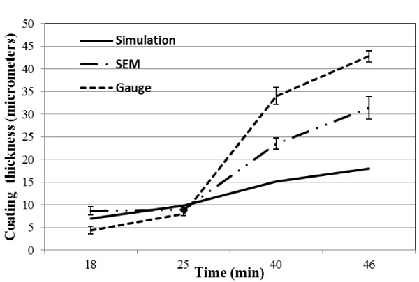
Figure 6. Simulated and experimental electroplating thickness vs. time at current density of 6.12 × 10² A/m2.
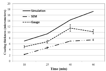
Figure 7. Simulated and experimental electroplating thickness vs. time at current density of 2.5 × 10² A/m2.
Effect of electrolyte conductivity on coating thickness
This experimental test was conducted with different electrical conductivities of the electrolyte keeping the other parameters constant (duration 46 mins and current density 3.57 × 10²(A/m2). The electrolyte conductivity evaluated were 4.23 S/m2, 1.9 S/m2, 0.93 S/m2 and 0.54 S/m2 on a 1.4 cm × 1.4 cm area of contact. The results from the experiment are tabulated in Table 3.
Table 3. Electrodeposition coating at varying electrolyte conductivities.
|
Thickness (micrometer) |
Conductivity (S/m2) |
4.23 |
1.9 |
0.93 |
0.54 |
Simulation |
17.6 |
6 |
2 |
1.6 |
Gauge |
11.8 ± 0.37 |
2 |
NA |
NA |
SEM |
13.45 ± 0.47 |
NA |
NA |
NA |
NA: coating not uniformity formed
Table 3 shows a decreasing trend in the simulated thickness coatings with decrease in the electrical conductivity of the electrolyte. Experimental determination of the coating under similar conditions resulted in a coating under one condition (4.23 S/m2), while the coating either was not uniformly formed or not formed at all under other conditions (1.9, 0.93 and 0.54 S/m2). Thus although the model accurately predicted the general trends, experimental observations indicated difficulties in forming a uniform coating at those electrolyte conductivities (1.9, 0.93 and 0.54 S/m2). Thus both the model and experiments indicates the requirement of appropriate electrolyte conductivity for the electrodeposition to occur. Lack of appropriate conductivity would hinder flow of ions within the electrolyte solution leading to difficulties in formation of a uniform coating.
In summary we have developed a mathematical model to simulate the electrodeposition of copper on cobalt-chrome alloy. At 30 min the model predicted the copper thickness to be 11.7 µm while experimentally the coating thickness was found to be 9.445+/-1.79 (mean +/- SD) using SEM and 12.375+/-1.36 (mean +/- SD) using thickness gauge. The relative accuracy of the predicted and experimental values validates our model. This demonstrates the preliminary applicability of the model in predicting electro deposition of copper on cobalt chrome substrate. When predicting effect of current density the model accurately predicts general trends however the model seems to vary from experimental values in regions where there is significant effect of the electrochemical double layer that the model does not account for. The model accurately predicts the trend of effect of electrolyte conductivity on coating formation. The model can thus be used as a starting point to predict effect of process parameters on electrodeposition thickness however modifications are needed to incorporate experimental realities not accounted for in the model.
This material is based upon work supported by the National Science Foundation under award Number EPS-0903806 and matching support from the State of Kansas through the Kansas Board of Regents. The authors would also like to acknowledge Wichita State University for partial financial support of materials and supplies for this work.
- Carolin K, Andreas B, Elham A (2013) Fundamental consolidation mechanisms during selective beam melting of powders. Model Simul Mat Sci Eng 21: 085011.
- Lee K, Fishwick PA (2001) Building a model for real-time simulation. Future Generation Computer Systems 17: 585-600.
- Kresse G, Hafner J (1994) Ab initio molecular-dynamics simulation of the liquid-metal amorphous-semiconductor transition in germanium. Phys Rev B Condens Matter 49: 14251-14269. [Crossref]
- Dickinson EJF, Ekström H, Fontes E (2014) COMSOL Multiphysics®: Finite element software for electrochemical analysis. A mini-review. Electrochem Comm 40: 71-74.
- Levytskyy A, Vangheluwe H, Rothkrantz LJM, Koppelaar H (2009) MDE and customization of modeling and simulation web applications. Simul Modelling Pract Theory 17: 408-29.
- Henderson SG, Nelson BL (2006) Chapter 1 Stochastic Computer Simulation. In: Shane GH and Barry LN, (eds.). Handbooks in Operations Research and Management Science. Elsevier, p. 1-18.
- Rinard IH (1996) Core models, coordinators, and connectors in the dynamic modeling and simulation of multiphase systems. Comput Chem Eng 20: S969-S74.
- Odette GR, Wirth BD, Bacon DJ, Ghoniem NM (2001) Multiscale-Multiphysics Modeling of Radiation-Damaged Materials: Embrittlement of Pressure-Vessel Steels. MRS Bull 26: 176-181.
- Altug Y, Wagner AB (2012) Source and Channel Simulation Using Arbitrary Randomness. IEEE Trans Inf Theory 58: 1345-60.
- Evstigneev IV, Schürger K (1994) A limit theorem for random matrices with a multiparameter and its application to a stochastic model of a large economy. Stoch Process Their Appl 52: 65-74.
- Tanaka H, Watada J (1988) Possibilistic linear systems and their application to the linear regression model. Fuzzy Sets and Systems 27: 275-289.
- Albrecht P (1983) Parametric multiple regression risk models: Theory and statistical analysis. Insurance: Mathematics and Economics 2: 49-66.
- Lai Y (2009) Adaptive Monte Carlo methods for matrix equations with applications. J Comput Appl Math 231: 705-14.
- Li Y, Chiang HD, Choi BK, Chen YT, Huang DH, et al. (2008) Load models for modeling dynamic behaviors of reactive loads: Evaluation and comparison. Int J Electr Power Energy Syst 30: 497-503.
- Meinert TS, Don Taylor G, English JR (1999) A modular simulation approach for automated material handling systems. Simul Modelling Pract Theory 7: 15-30.
- Datta A, Rakesh V (2009) An Introduction to Modeling of Transport Processes. Cambridge University Press.
- Basile A, Bhatt AI, O’Mullane AP, Bhargava SK (2011) An investigation of silver electrodeposition from ionic liquids: Influence of atmospheric water uptake on the silver electrodeposition mechanism and film morphology. Electrochimica Acta 56: 2895-2905.
- Zheng Z, Stephens RM, Braatz RD, Alkire RC, Petzold LR (2008) A hybrid multiscale kinetic Monte Carlo method for simulation of copper electrodeposition. J Comput Phys 227: 5184-5199.
- Mahapatro A, Kumar SS (2015) Determination of Ionic Liquid and Magnesium Compatibility via Microscopic Evaluations. J Adv Microsc Res 10: 89-92.
- Abdel-Fattah TM, Loftis JD, Mahapatro A (2015) Nanoscale Electrochemical Polishing and Preconditioning of Biometallic Nickel-Titanium Alloys. Nanosci Nanotechnol 5: 36-44.
- Lou HH, Huang YL (2003) Hierarchical decision making for proactive quality control: system development for defect reduction in automotive coating operations. Eng Appl Artif Intell 16: 237-250.
- Mette A, Schetter C, Wissen D, Lust S, Glunz SW, et al. (2006) Increasing the Efficiency of Screen-Printed Silicon Solar Cells by Light-Induced Silver Plating. Photovoltaic Energy Conversion, Conference Record of the 2006 IEEE 4th World Conference on. p. 1056-1059.
- Wanping C, Longtu L, Zhilun G (1997) Effects of Electroless Nickel Plating on Resistivity-temperature Characteristics of (Ba1-xPbx)TiO3thermistor. J Mater Res 12: 877-879.
- Krumbein S, Antler M (1968) Corrosion Inhibition and Wear Protection of Gold Plated Connector Contacts. IEEE Transactions on Parts, Materials and Packaging 4: 3-11.
- Mandin P, Fabian C, Lincot D (2006) Importance of the density gradient effects in modelling electro deposition process at a rotating cylinder electrode. Electrochimica Acta 51: 4067-4079.
- Deconinck J (1994) Mathematical modelling of electrode growth. J Appl Electrochem 24: 212-8.
- Hughes M, Strussevitch N, Bailey C, McManus K, Kaufmann J, et al. (2010) Numerical algorithms for modelling electrodeposition: Tracking the deposition front under forced convection from megasonic agitation. Int J Numer Methods Fluids 64: 237-268.
- Obaid N, Sivakumaran R, Lui J, Okunade A (2013) Modelling the Electroplating of Hexavalent Chromium. COMSOL Conference. Boston, USA.
- Hughes M, Bailey C, McManus K (2007) Multi Physics Modelling of the Electrodeposition Process. Thermal, Mechanical and Multi-Physics Simulation Experiments in Microelectronics and Micro-Systems, 2007. EuroSime 2007 International Conference on. Pp: 1-8.
- Bird RB, Stewart WE, Lightfoot EN (2007) Transport phenomena. New York: John Wiley and Sons, pp.780.
- Martell AE (1946) Entropy and the second law of thermodynamics. J Chem Educ 23: 166.
- Lu X (1997) Application of the Nernst-Einstein equation to concrete. Cem Concr Res 27: 293-302.
- Cai J, Jin C, Yang S, Chen Y (2011) Logistic distributed activation energy model – Part 1: Derivation and numerical parametric study. Bioresour Technol 102: 1556-1561.
- Seyedi H, Abam Z and Golabi S (2012) Comprehensive Analysis of the Impacts of Different Parameters on Transmission Line Switching Overvoltages. International Review on Modelling and Simulations 5: 2174-2182.
- Noren DA, Hoffman MA (2005) Clarifying the Butler–Volmer equation and related approximations for calculating activation losses in solid oxide fuel cell models. J Power Sources 152: 175-181.
- Kamata M, Paku M (2007) Exploring Faraday's Law of Electrolysis Using Zinc–Air Batteries with Current Regulative Diodes. J Chemi Educ 84: 674.
- Marichev VA (1991) A new possibility of application of electron tunneling effects in electrochemical double layer structure investigations. Surface Science 250: 220-228.
- Su YZ, Fu YC, Wei YM, Yan JW, Mao BW (2010) The Electrode/Ionic Liquid Interface: Electric Double Layer and Metal Electrodeposition. ChemPhysChem 11: 2764-2778.
- Shi H (1996) Activated carbons and double layer capacitance. Electrochimica Acta 41: 1633-1639.