The relationship between single nucleotide polymorphisms (SNPs) and phenotypes is noisy and cryptic due to the abundance of genetic factors and the influence of environmental factors on complex traits, which makes the idea of applying artificial neural networks (ANNs) as universal approximates of complex functions promising.
In this study, we compared different ANN architectures and input parameters to predict the adult length of Pacific lampreys, which is the primary indicator of their total migratory distance. Feedforward and simple recurrent network architectures with a different range of input parameters and different sizes of hidden layers were compared. Results indicate that the highest performing ANN had an accuracy of 67.5% in discriminating between long and short specimens. Sensitivity and specificity were 62.16% and 70.73%, respectively.
Our results imply that feedforward ANN architecture with a single hidden neuron is enough to solve the problem of specimen classification. Nonetheless, while ANNs are useful at approximating functions with unknown relationships in the case of SNP data, additional work needs to be performed to ensure that the chosen SNP markers are related to functional regions related to the examined trait, as the use of non-specific markers will result in the introduction of noise into the dataset
artificial neural network, single nucleotide polymorphism, pacific lamprey, genetic marker
Migratory behavior is the long-distance movement of individuals, which mostly occurs on a seasonal basis. As one of the most well-known and studied phenomena in behavioral biology, migratory behavior can be observed in most animal species. Animals with unpredictable migratory patterns represent a challenge to ecologists working on effective population management and conservation, as their movement patterns are influenced by multiple events spread across a wide geographic range, often encompassing international borders [1]. The signals that start migratory behavior are largely environmental and are usually related to the length of day in bird species, or the water temperature in fish migration. However, there is evidence that genetics plays an important role in the migratory predisposition of individuals [2]. The genetic molecular mechanisms regulating migratory behavior have already been studied in birds, and genes that control such behavior have been discovered [3].
Single nucleotide polymorphisms (SNPs) have previously been used to predict a variety of traits in numerous species, ranging from quantitative [4,5], to discrete traits, such as eye color [6]. SNPs are single base sequence variations between individuals at a specific position in the genome. They are abundant in the genome of humans and animals, and are commonly used to differentiate between individuals of a species [7].
The Pacific lamprey (Entosphenus tridentatus) has recently been studied [8] regarding SNP markers that could be used to predict the migratory behavior of an individual. In that study, three SNP markers that can be used as efficient predictors of migratory behavior in this species have been elucidated. The main characteristic found to be indicative of the migratory behavior of such individuals was the total body length, as it was noticed that shorter fish are less likely to exhibit long distance migratory behavior [8]. Pacific lampreys have an important role in the ecosystem, serving as a buffer for salmon from predators and acting as an important sustenance food and cultural symbol for many tribes living along the Pacific coast [9]. Pacific lampreys are a highly dispersive, anadromous type of fish, which lacks a strict homing site. Instead, Pacific lampreys seem to locate their spawning sites based on pheromonal cues [10,11]. This makes the ability to predict their movements and migratory behavior both challenging and important from a conservatory perspective. The population of Pacific lampreys is on the decline due to environmental issues, inadequate dam design impeding their spawning migration, and prejudice caused by the popular opinion that lampreys are an invasive parasitic species, despite being indigenous to the Pacific coastal area [12,13]. Their migratory behavior has previously been studied using passive integrated transponder (PIT) tagging, where the correlation with migratory distance and length was observed in adult specimens [14].
Artificial neural networks are attractive for applications in genetics [15-18], as the relationship between SNPs and phenotypes is noisy and cryptic due to the abundance of genetic factors and the influence of environmental factors on complex traits [19,20]. They are applicable to various biological problems for categorization, such as discriminating between wild and domesticated populations of salmon and trout, as well as regression problems, such as predicting the sulphur removal by Acidithiobacillus species [21,22].
This study compares the predictive ability of two different neural network architecture types, a varying number of hidden nodes, as well as different input parameters and training data distributions. The target parameter is the total adult body length of individual Pacific lampreys, and is based on a previously published [8].
For problems of this type, the most frequently used ANNs are linear feedforward, and recurrent (feedback architecture), such as the Elman neural network [23-25]. Therefore, we have made a direct comparison of the neural network types on identical datasets to determine which is most suitable for predicting a phenotypical trait based on SNP data.
Feedforward networks
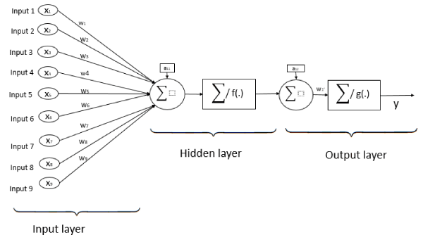
Single layer feedforward networks are frequently used for regression problems and forecasting. A linear feedforward neural network is often sufficient to properly perform classification tasks and is also applicable to regression tasks [26-28]. They are models in which information travels in one direction without any loops or cycles between the input and output. Neurons are assigned random weights at the beginning, and the sum of the products (linear combination) of the weights and inputs is calculated at each neuron. If the value obtained is greater than a given threshold value, the neuron “fires” and assumes the activated value. If the threshold is not reached, it assumes a deactivated value. The training of a network depends on outputs obtained. In the case of using the delta rule, the error is calculated between the predicted and target data, and the weights of the neurons are adjusted based on the error. This “backpropagation” process is repeated until a sufficiently low level of error is reached, or until a predefined cutoff point is reached [29]. A representation of a feedforward neural network with one neuron in the hidden layer, and nine input neurons is shown in Figure 1.

Figure 1. Single layer Feedforward neural network architecture with nine inputs, one neuron in hidden layer, and one neuron in output layer.
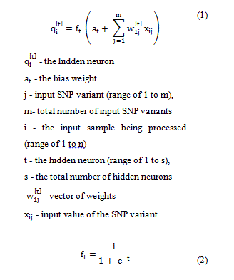
In this study, the input to each hidden neuron is a linear combination of a vector of weights, input SNP variants and a “bias” weight for the feedforward networks. The input to each neuron is obtained as represented in Equation 1. The result is then transformed via the sigmoid activation function (Equation 2) to produce the hidden neurons output value.

The output layer consists of neurons as well. The inputs to neurons in the output layer is a linear combination of outputs of neurons in the hidden layer, weights of the output layer q, and an output layer bias neuron b. The value obtained is transformed by the linear transformation function pt(.) to generate the value of the predicted adult length of an individual, as presented in Equation 3.

During the training of the neural network, the optimal weights are established using the Levenberg-Marquardt algorithm (LMA), which is commonly used for training ANNs [30,31], and which minimizes the error between the predicted and the actual weight [32]. This is performed by using a process of backpropagation that continues until an optimal mean error squared level is reached or stopping criteria was fulfilled.
Elman neural networks
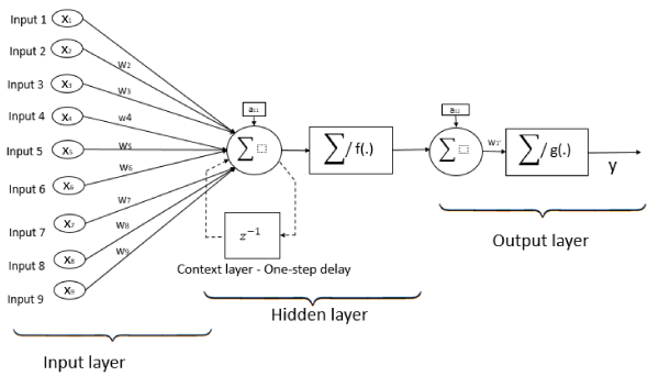
Elman neural networks have feedback architecture and are also referred to as recurrent neural networks. This architecture, in addition to the layers found in the feedforward network architecture, also has a “context” layer which saves the unweighted outputs of the previous iterations hidden layer, thus giving the neural network a sort of short term memory, or context that feedforward networks do not possess [33]. Elman networks are identical to feedforward ones in their first iteration, due to no context layer being present. After the first iteration, the context layer is formed by the previous iterations of the hidden layer, thus resembling a three-layer feedforward network, with one layer being a copy of the previous iterations hidden layer. A representation of an Elman network with one hidden neuron, and nine input neurons is shown in Figure 2.

Figure 2. Elman (Recurrent) neural network architecture with nine inputs, one neuron in hidden layer, and one neuron in output layer.
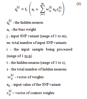
Equation 4 was used to calculate the hidden neuron values in the Elman networks; it is very similar to Equation 1 with the only difference being the addition of the context layer inputs.

The sigmoid function (Equation 2) was used as the activation function in the hidden layer, with the linear transformation function (Equation 3) being used as the activation function in the output layer.
The Elman network was trained using the Gradient Descent with Momentum & Adaptive Learning Rate training method, which is a backpropagation algorithm commonly used for training recurrent ANNs [34]. The training continued until a minimal level of error was reached, or stopping criteria was fulfilled.
Dataset creation
A dataset containing 797 individuals that were genotyped for 94 total markers has been collected [8], with additional data describing their size, weight and migratory distance travelled. Three of those markers were determined to have a correlation with total adult length, and were found to be linked to genes with association to morphological traits (Table 1).
Table 1. Association of SNP markers to morphological traits.
SNP Marker |
Morphological Trait |
Etr_5317 |
Localizes to DYM gene which encodes a protein associated with normal skeletal development and brain function. |
Etr_4281 |
aligned to the human homologue PCDH15 that encodes a membrane protein which functions to mediate calcium-dependent cell-cell adhesion. |
Etr_1806 |
Does not appear to localize within any described gene region. |
In order to compare the effects of SNP markers that have no direct correlation to the predicted trait, we have constructed three separate datasets. One dataset contained only the SNP markers that were determined to be related to adult length (dataset S3). A second dataset containing the S3 SNPs and seven arbitrarily chosen SNPs (S10), and a dataset containing all SNPs included in the study (S94). Since SNPs cannot be represented as continuous variables, and since each SNP has multiple possible variants in which it appears, each variant was used as a flag value, totaling in the neural networks having three times the number of SNPs as input neurons. An exception was the S94 dataset, which contained two SNPs that had two variants instead of three, resulting in a total of 280 input neurons. An example of this is shown in Table 2. The target value in the datasets was the total length of the individual.
Table 2. Coding of input parameters of ANN.
Etr_1806 |
Etr_1806_aa |
Etr_1806_ag |
Etr_1806_gg |
AA |
1 |
0 |
0 |
AG |
0 |
1 |
0 |
GG |
0 |
0 |
1 |
In order to investigate what effect the distribution of the test data has on the training of the neural network, we have devised three different schemes of splitting the data, H, T and Q, described in Table 3. In total, this resulted in nine different input and test datasets.
Table 3. Data splitting schemes for the datasets used in this study. Data were divided based on length of the individual samples. Training datasets are represented in the top, while corresponding testing data splits are represented in the bottom part of the table.
Training dataset |
H split |
T split |
Q split |
Number of samples |
Length |
Number of samples |
Length |
Number of samples |
Length |
300 |
<660 mm |
200 |
≤ 610 mm |
150 |
<610 mm |
300 |
≥ 660 mm |
200 |
>610 mm and ≤ 655 mm |
150 |
>610 mm and ≤ 650 mm |
|
|
200 |
>655 mm |
150 |
>650 mm and ≤ 685 mm |
|
|
|
|
150 |
>685 mm |
Testing dataset |
H split |
T split |
Q split |
Number of samples |
Length |
Number of samples |
Length |
Number of samples |
Length |
145 |
<660 mm |
6 |
≤ 610 mm |
56 |
less than 610 mm |
52 |
≥ 660 mm |
39 |
>610 mm and ≤ 655 mm |
89 |
>610 mm and ≤ 650 mm |
|
|
152 |
>655 mm |
38 |
>650 mm and ≤ 685 mm |
|
|
|
|
41 |
>685 mm |
The output value of the ANNs is the length of the individual expressed in millimeters. This output value is normalized to values between 0 and 1 (Equation 5), as this is a standard procedure done in order to obtain better initial weights and make the training faster (Larose 2014).

In Equation 5, the minimum length of fish in the training dataset is 480 mm, while the maximum length of fish in the dataset is 770 mm.
Neural network training and performance measurement
We examined the accuracy and performance of neural networks that employed the feedforward architecture with the Levenberg-Marquardt training method, and the recurrent neural network architecture, also known as Elman architecture, with the Gradient Descent with Momentum and Adaptive Learning Rate training algorithm. Both are popular optimization algorithms used in the ANN domain, and are the default algorithms used in MATLAB for feedforward, and Elman networks, respectively [35]. The number of hidden neurons, as well as different input values, and training dataset distributions were examined. The number of neurons in the hidden layer was repeatedly increased by a single neuron, starting at one and continuing to twenty hidden neurons, which we have chosen as an arbitrary stopping point.
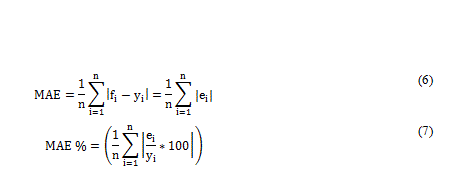
Mean absolute error (MAE) and Pearson’s correlation coefficients were used to measure the ANN predictive performance. The Mean absolute error was calculated based on equations (6) and (7).


Pearson’s correlation coefficient of the predicted and actual values (r) was calculated as a measure of linearity between input and output values using Equation 8, where n is the total number of samples (Table 4).
Table 4. Neural network testing results.
Mean Absolute Error |
Mean Absolute Error (%) |
Pearsons Correlation
Coefficient |
Accuracy in % for
categorical division |
30.16 mm |
% |
0.68 |
67.51% |

Each neural network was trained using 600 samples, and a 70:30 data split, with 70% of the data being used for training, and 30% being used for validation. The sampling was random in order to avoid any selection bias in the dataset. Performance testing was done with 197 samples that were not used during the training phase. This is a common data splitting scheme, frequently used in ANN applications [36].
This process was repeated for each network type using the three datasets, and three different data splits for each dataset, resulting in a total of 360 neural networks analyzed in this study. Data preprocessing and analysis were performed using the R programming language [37], while the construction and training of neural networks was performed using MATLAB [38].
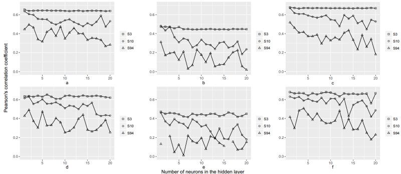
The combined results of this study can be seen in Figure 3. It plots the correlation of the target and predicted parameter for all datasets and data splits. The individual plots (a-f) represent the correlations of the target and predicted parameters for the different data splits. The first row (a-c) represents the results of using the Elman architecture, while the second row (d-f) represents the results of using the feedforward architecture.

Figure 3. Training performances of Feedforward and Recurrent Neural Network architectures with different dataset distribution and number of neurons in the hidden layer. The first row (a-c) represents the Elman networks, the second row (d-f) represents feedforward networks. The blank squares are the S3 dataset networks, S10 is represented by blank circles, while S94 is represented by blank triangles. The first column is split according to the H scheme, second column is the T scheme, while the third column is the Q scheme. The vertical axis is the Pearsons r coefficient, while the horizontal axis represents the number of neurons in the hidden layer.
Predictive ability of different ANN architectures
In the case of Elman networks, no improvement was observed with the increase of the number of neurons in the hidden layer. Their performance decreased rapidly once the hidden layer exceeded three neurons, especially in the case of noisy datasets, while in the case of noise-free ones, the performance stays consistent (Figure 3a-3c). The explanation for such a fall in accuracy is that the increase in hidden nodes resulted in overfitting, that is, the neural network memorized the training data, but did not learn the underlying rules that would enable it to predict the length of new samples [35].
Feedforward networks exhibited no great changes in their performance with the increase of neurons in the hidden layer in the S3 dataset. However, in the noisy datasets S10 and S94, the increase of the number of neurons served to handle the noisy inputs and increased performance. This is most evident in S94, where the highest performing feedforward neural networks had two, seven, and four neurons in the hidden layer, respectively (Figure 3d-3f).
In a general comparison of Elman and feedforward neural network architectures, Elman shows more consistency in its predictive ability when the number of neurons is changed in the hidden layer. However, it should be noted that the highest correlation was obtained by a single neuron feedforward network utilizing the S3 dataset with the Q data splitting scheme.
Predictive ability according to training data
The S3 dataset consistently provided the best results as the SNPs used in this scenario have been previously correlated to the target variable, thus providing a noise-free dataset, and being ideal input variables. The S10 dataset performed comparably to the S3 dataset in neural networks with a small hidden layer, while the performance of the S94 dataset was erratic at best. The Q data splitting scheme (Table 3) provided the best results, despite the performance of neural networks worsening as the size of the hidden layer started to exceed ten neurons. The H data split was a close second, while the T data split exhibited the worst performance of the three, regardless of number of hidden neurons or network architecture used.
Highest performing feedforward ANN testing
The testing of the highest performing ANN was performed with 197 samples that were not included in the training dataset (Table 3). The performance of the trained feedforward ANN for the test dataset was measured by mean absolute error (Equations 6 and 7). A mean absolute error of 30.162 mm was achieved. When converted to percentage values, the mean absolute error was 5.03% (Equation 2, Table 4).
The Pearson correlation coefficient was calculated to be 0.68 for the test dataset, which leads to the conclusion that a relatively high level of correlation between the true and predicted lengths of the samples was achieved. The network had an accuracy of 67.5% in discriminating between long and short specimens. The accuracy was calculated by transforming the true and predicted values from the test dataset into categorical ones, those being either long (≥ 660mm) or short. Out of 197 samples in the test set, 74 were from group long and 123 were from group short. Out of 74 long samples, 46 samples were correctly predicted giving the sensitivity of 62.16%. Out of 123 short samples, 87 were correctly predicted giving the specificity of 70.73% (Table 5).
Table 5. Performance of the expert system.
|
Predicted condition |
|
True condition |
Long |
Short |
% of true predictions |
% of false predictions |
Long (≥ 660 mm) 74 |
46 |
28 |
62.16 |
38.84 |
Short (<660 mm) 123 |
87 |
36 |
70.73 |
29.27 |
2021 Copyright OAT. All rights reserv
Changing environmental circumstances influences the natural migratory instincts in Pacific lampreys and causes them to travel great distances in order to reach their natural spawning sites. In this paper, we present a comparison between simple recurrent (Elman) neural networks and feedforward networks for the prediction of the adult body size of Pacific lamprey individuals according to their genotypes. The feedforward architecture proved to be efficient in classifying the phenotype of individuals according to the SNP variations of three markers.
A three-centimeter average difference between the actual and the predicted length of an individual obtained in the results is satisfactory for a species where the average size of an individual is about 55 cm. However, as promising as the results appear to be, one must take into consideration the inherent difficulty of predicting a complex trait that is largely influenced by environmental factors, not just genetic ones. The size of Pacific lampreys at adulthood is heavily dependent on environmental factors such as water temperature [39] which have not been accounted for in this study, as the source dataset did not delve into such elements.
The results were compared to similar studies, where regression model and artificial neural networks were used with SNP data. A constructed multinomial logistic regression model is designed using 24 SNPs from eight genes. The proposed model revealed the accuracy for predicting intermediate eye color of 0.73 [40]. On the other hand, prediction of eye color using multinomial regression model based on six IrisPlex SNPs shown the accuracy of 0.796 for intermediate eye color [6]. Also, regression model found its application in trait prediction using whole-genome sequencing data. The results shown the reidentification accuracy of different pool sizes range from 0.075 to 0.85 for eye color trait [41].
However, in ANN it was found that they are in line, or even outperform certain other studies by a small margin, depending on the dataset. SNP data were used to predict childhood allergic asthma in humans, and the obtained accuracy was 74.4%, which is comparable to the results obtained in the present study after transforming the output to a categorical value where the accuracy of predicting whether the individual is a large fish (length >66 cm) was 67.5% [42].
An ANN was used to predict various complex traits in cattle, and the obtained predictive correlation ranged from 0.47, to the best-case scenario of 0.67, whereas the correlation coefficient in the present study matched theirs being 0.68. These results being in line with previous research give the authors confidence in the test design and execution of the ANN in this study, and serve as another set of evidence as to the effectiveness of using ANN in combination with SNPs to predict complex traits [15].
The performance of different architectures of neural networks was compared with the task of predicting phenotypes of cattle and wheat, and the obtained conclusion was that nonlinear ANN outperform linear architectures in that scenario, as they had higher predictive correlations. Our results outperformed their predictive values, possibly due to our use of SNPs known to be involved in the targeted trait, while they used a large SNP panel, which might have had the unwanted side-effect of introducing noise into the dataset [16].
A multitude of ANN models was explored for the prediction of marbling score in Angus cattle. The authors used different training algorithms, different activation functions and different numbers of neurons in hidden layers, and obtained a high correlation in their training set ranging from 0.776 to 0.858, depending on the algorithm and input dataset used. As they used SNP panels of 3,000 and 700 markers, it remains to be explored whether their results could have been improved by limiting the number of input SNPs to only the most relevant ones, and the application of their methods to the dataset used in our study would be a good topic for further research [17].
ANNs with relatively small numbers of hidden neurons showed good results in our study, which is not uncommon, as even single hidden neuron ANNs have the ability to learn complex rules [43,44]. The increase in the number of hidden neurons only became necessary in the case of noisy datasets, where it served to handle the noisy data. The greatest influence on the performance of the neural network came from the choice of input values, and distribution of values in the input dataset, as the best performance was achieved by a training data split where the lengths of the individual samples were evenly distributed.
We have compared a number of ANN models for the prediction of a phenotypic trait, based on SNP data. We have investigated the effects of network architecture, hidden layer sizes, inputs, and training data splits in order to obtain the highest performing neural network model for the prediction of adult Pacific lamprey length. The results indicate that using a minimal number of inputs in the dataset (three) with a one neuron in the hidden layer and the feedforward neural network architecture provides the most accurate predictive performance. These results correlate with previous findings in this area.
While artificial neural networks are great at approximating unknown relationships, they work much better in the absence of noise in the dataset in the case of a SNP panel, and any such further studies must be initiated with an exploration of the relevancy of the chosen inputs to the output traits in order to avoid noisy data.
The dataset(s) supporting the conclusions of this article is (are) available in the Data Dryad repository, http://datadryad.org/resource/doi:10.5061/dryad.t0391.
LB: Designed the experimental set-up, wrote the manuscript. IM: performed the data mining, and analysis. AA, AC & LG: Contributed to the manuscript. AB: Coordinated the study and provided critical insights. All authors read and approved the final manuscript.
- Martin TG, Chadès I, Arcese P, Marra PP, Possingham HP, et al. (2007) Optimal conservation of migratory species. PLoS One 2: e751. [Crossref]
- Skov C, Aarestrup K, Baktoft H, Brodersen J, Brönmark C, et al. (2010) Influences of environmental cues, migration history, and habitat familiarity on partial migration. Behav Ecol 21: 1140-1146.
- Mueller JC, Pulido F, Kempenaers B (2011) Identification of a gene associated with avian migratory behaviour. Proc Biol Sci 278: 2848-2856. [Crossref]
- Morota G, Abdollahi-Arpanahi R, Kranis A, Gianola D (2014) Genome-enabled prediction of quantitative traits in chickens using genomic annotation. BMC Genom 15: 109. [Crossref]
- Yang J, Benyamin B, McEvoy BP, Gordon S, Henders AK, et al. (2010) Common SNPs explain a large proportion of the heritability for human height. Nat Genet 42: 565-569. [Crossref]
- Kastelic V, PoÅ›piech E, Draus-Barini J, Branicki W, DrobniÄ K (2013) Prediction of eye color in the Slovenian population using the IrisPlex SNPs. Croat Med J 54: 381-386. [Crossref]
- Butler JM (2011) Advanced topics in forensic DNA typing: methodology. Academic Press, Cambridge.
- Hess JE, Caudill CC, Keefer ML, McIlraith BJ, Moser ML, et al. (2014) Genes predict long distance migration and large body size in a migratory fish, Pacific lamprey. Evol Appl 7: 1192-1208. [Crossref]
- Close DA, Fitzpatrick MS, Li HW (2002) The ecological and cultural importance of a species at risk of extinction, Pacific lamprey. Fisheries 27: 19-5.
- Hess JE, Campbell NR, Close DA, Docker MF, Narum SR (2013) Population genomics of Pacific lamprey: adaptive variation in a highly dispersive species. Mol Ecol 22: 2898-2916. [Crossref]
- Spice EK, Goodman DH, Reid SB, Docker MF (2012) Neither philopatric nor panmictic: microsatellite and mtDNA evidence suggests lack of natal homing but limits to dispersal in Pacific lamprey. Mol Ecol 21: 2916-2930. [Crossref]
- Jackson A, Moser M (2012) Low-elevation dams are impediments to adult Pacific lamprey spawning migration in the Umatilla River, Oregon. North Am J Fish Manag 32: 548-556.
- Moser ML, Close DA (2003) Assessing Pacific lamprey status in the Columbia River basin. Northwest Sci 77: 116-125.
- Keefer ML, Moser ML, Boggs CT, Daigle WR, Peery CA (2009) Effects of body size and river environment on the upstream migration of adult Pacific lampreys. North Am J Fish Manag 29: 1214-1224.
- Ehret A, Hochstuhl D, Gianola D, Thaller G (2015) Application of neural networks with back-propagation to genome-enabled prediction of complex traits in Holstein-Friesian and German Fleckvieh cattle. Genet Sel Evol 47: 22. [Crossref]
- Gianola D, Okut H, Weigel KA, Rosa GJ (2011) Predicting complex quantitative traits with Bayesian neural networks: a case study with Jersey cows and wheat. BMC Genet 12: 87. [Crossref]
- Okut H, Wu XL, Rosa GJ, Bauck S, Woodward BW, et al. (2013) Predicting expected progeny difference for marbling score in Angus cattle using artificial neural networks and Bayesian regression models. Genet Sel Evol 45: 34. [Crossref]
- Aljovic A, Badnjevic A, Gurbeta L (2016) Artificial Neural Networks in the Discrimination of Alzheimer's disease Using Biomarkers Data. IEEE 5th Mediterranean Conference on Embedded Computing (MECO), Bar, Montenegro.
- MacKay DJ (2003) Information theory, inference and learning algorithms. Cambridge university press, Cambridge.
- Secerovic A, Gurbeta L, Omanovic-Miklicanin E, Badnjevic A (2017) Genotype Association with Sport Activity: The Impact of ACE and ACTN3 Gene Polymorphism on Athletic Performance. Int J Eng Res Technol.
- Acharya C, Mohanty S, Sukla LB, Misra VN (2006) Prediction of sulphur removal with Acidithiobacillus sp. using artificial neural networks. Ecol Model 190: 223-230.
- Hansen MM, Kenchington E, Nielsen EE (2001) Assigning individual fish to populations using microsatellite DNA markers. Fish Fish 2: 93-112.
- Hu X, Maglia A, Wunsch D (2005) A general recurrent neural network approach to model genetic regulatory networks. Conf Proc IEEE Eng Med Biol Soc 5: 4735-4738. [Crossref]
- Ramos EG, Martínez FV (2013) A Review of Artificial Neural Networks: How Well Do They Perform in Forecasting Time Series? Analítika Rev Análisis Estad 6: 7-18.
- Veljovic E, Spirtovic-Halilovic S, Muratovic S, Osmanovic A, Badnjevic A, et al. (2017) Artificial Neural Network and Docking Study in Design and Synthesis of Xanthenes as Antimicrobial Agents. IFMBE Proceedings 62: 617-626.
- Badnjevic A, Cifrek M, Koruga D, Osmankovic D (2015) Neuro-fuzzy classification of asthma and chronic obstructive pulmonary disease. BMC Med Inform Decis Mak 15: S1. [Crossref]
- Byvatov E, Fechner U, Sadowski J, Schneider G (2003) Comparison of support vector machine and artificial neural network systems for drug/nondrug classification. J Chem Inf Comput Sci 43: 1882-1889. [Crossref]
- Khan J, Wei JS, Ringner M, Saal LH, Ladanyi M, et al. (2001) Classification and diagnostic prediction of cancers using gene expression profiling and artificial neural networks. Nat Med 7: 673-679. [Crossref]
- Larose DT (2014) Discovering knowledge in data: an introduction to data mining. John Wiley & Sons, Hoboken.
- Yu H, Wilamowski BM (2011) Levenberg–marquardt training. Ind Electron Handb 5: 1.
- Alic B, Sejdinovic D, Gurbeta L, Badnjevic A (2016) Classification of Stress Recognition using Artificial Neural Network. IEEE 5th Mediterranean Conference on Embedded Computing (MECO), Bar, Montenegro.
- Fojnica A, Osmanovic A, Badnjevic A (2016) Dynamical Model of Tuberculosis-Multiple Strain Prediction based on Artificial Neural Network. IEEE 5th Mediterranean Conference on Embedded Computing (MECO), Bar, Montenegro.
- Elman JL (1990) Finding structure in time. Cogn Sci 14: 179-211.
- Moreira M, Fiesler E (1995) Neural networks with adaptive learning rate and momentum terms. Idiap.
- Hagan MT, Menhaj MB (1994) Training feedforward networks with the Marquardt algorithm. IEEE Trans Neural Netw 5: 989-993. [Crossref]
- Reitermanova Z (2010) Data splitting. WDS’s 10 Proc Contrib Pap Part 10: 31-36.
- Dean CB, Nielsen JD (2007) Generalized linear mixed models: a review and some extensions. Lifetime Data Anal 13: 497-512. [Crossref]
- Demuth H, Beale M (1993) Neural network toolbox for use with MATLAB.
- Griffiths RW, Beamish F, Morrison B, Barker L (2001) Factors affecting larval sea lamprey growth and length at metamorphosis in lampricide-treated streams. Trans Am Fish Soc 130: 289-306.
- Liu F, van Duijn K, Vingerling JR, Hofman A, Uitterlinden AG, et al. (2009) Eye color and the prediction of complex phenotypes from genotypes. Curr Biol 19: R192-R193. [Crossref]
- Lippert C, Sabatini R, Maher MC, Kang EY, Lee S, et al. (2017) Identification of individuals by trait prediction using whole-genome sequencing data. Proc Natl Acad Sci U S A 114: 10166-10171. [Crossref]
- Tomita Y, Tomida S, Hasegawa Y, Suzuki Y, Shirakawa T, et al. (2004) Artificial neural network approach for selection of susceptible single nucleotide polymorphisms and construction of prediction model on childhood allergic asthma. BMC Bioinform 5: 120. [Crossref]
- Nejjari H, Benbouzid MEH (2000) Monitoring and diagnosis of induction motors electrical faults using a current Park’s vector pattern learning approach. IEEE Trans Ind Appl 36: 730-735.
- Sarkisyan KS, Bolotin DA, Meer MV, Usmanova DR, Mishin AS, et al. (2016) Local fitness landscape of the green fluorescent protein. Nature 553: 397-401. [Crossref]

