Abstract
Over 50 years ago, Professor Edwards Lorenz of MIT illustrated the sensitive dependence of numerical solutions on initial conditions (ICs), known as chaos or a butterfly effect of the first kind. The equations he used have been referred to as the three-dimensional Lorenz model (3DLM). While the 3DLM has been extensively examined to illustrate the role of nonlinearity in producing chaos, higher-dimensional Lorenz models have been studied in order to understand the impact of increased degrees of nonlinearity on system stability. Compared to the 3DLM, the 5D or 6D Lorenz model (5DLM or 6DLM) requires a larger normalized Rayleigh parameter (r) for the onset of chaos (e.g., Shen, 2014; 2015). Mathematical analysis suggests that negative nonlinear feedback associated with additional small-scale modes in the 5D or 6DLM can effectively stabilize solutions. Here, to aid understanding regarding whether nonlinear feedback can be incorporated with one or two additional (parameterized) terms, a revised 3DLM is proposed for emulating the negative nonlinear feedback resolved by the 5DLM. For chaotic solutions, the critical value of the normalized Rayleigh parameter (rc) in the revised 3DLM (~52.1) is larger than that of the 3DLM (rc~24.74); and is comparable to but larger than therc of the corresponding 5DLM (~42.9). The result suggests that the stability of the revised 3DLM is overestimated between 43 ˂ r ˂ 52 as compared to the 5DLM. For stable solutions, the revised 3DLM produces the same steady-state (equilibrium-state) solutions as those in the 5DLM, when parameters are kept the same in both models (e.g.,r = 35). The revised 3DLM is unable to accurately depict the evolution of transient solutions in both amplitudes and phases, as compared to the 5DLM, but the trend mode of its transient solution is comparable to that of the 5DLM. The trend mode is determined as the non-oscillatory component of the solution using the parallel version of the ensemble Empirical Model Decomposition (EMD) algorithm. In addition, with the revised 3DLM, the dependence of the equilibrium-state solution on the implementation of the parameterized term suggests the importance of emulating the nonlinear (horizontal and vertical) advection of temperature into the parameterized term. Characteristics of the solution (such as overestimated stability, lack of detailed evolution, and a comparable trend mode) also appear in a different revised 3DLM with parameterized terms using the 6DLM.
Introduction
In his pioneering modeling paper published in 1963, Professor Edwards Lorenz of MIT illustrated the sensitive dependence of numerical solutions on initial conditions (ICs) using a very elegant set of nonlinear ordinary differential equations [1]. The numerical phenomenon of a solution’s dependance on ICs, appearing as the normalized Rayleigh parameter (r) exceeds a critical value ofrc, is now known as chaos or a butterfly effect of the first kind [2]. The equations are referred to as the (three-dimensional) Lorenz model (3DLM). Since the theory’s introduction by Lorenz, researchers have suggested that the source of chaos in the 3DLM is nonlinearity [3-6]. Various researchers have inferred that (1) small-scale processes can have a huge impact on large-scale processes (say, leading to the generation of a tornado) and (2) increased degrees of nonlinearity may further increase the degree of chaotic behavior. In regards to the generation of large-scale systems (e.g., a tornado), the process is referred to as a butterfly effect of the second kind [2], while the sensitive dependence of numerical solutions on ICs is called a butterfly effect of the first kind. However, Pielke [4]indicated that the inferred statements may not be accurate, and research shows that nonlinear feedbacks associated with newly added modes can be positive or negative [2,7]. In other words, nonlinear feedbacks associated with small-scale modes can either stabilize or destabilize solutions, consistent with view of Lorenz [8]on the role of small-scale processes: If the flap of a butterfly’s wings can be instrumental in generating a tornado, it can equally well be instrumental in preventing a tornado.
The 3DLM was derived from governing equations for 2D Rayleigh-Benard convection, which have two nonlinear advection terms,
 and
and  , here,
  is the streamfunction, and
  is the temperature perturbation.. However, only the impact of the latter is included in the 3DLM. In other words, nonlinearity in the 3DLM involves only nonlinear advection of temperature. The nonlinear interaction of two wave modes, which is expressed by the Jacobian term, can generate or impact a third wave mode through a downscale (or upscale) transfer process. The third wave mode can provide feedback to the incipient wave mode(s) via its subsequent upscale (or downscale) transfer process. Downscale and upscale transfer processes associated with the third mode form a nonlinear feedback loop that can be continuously extended when new modes are continuously generated. Appendix B of Shen [2] summarizes the successive downscale and upscale transfer processes via the Jacobian term,
  . Related discussions suggest that an ideal numerical model should include an infinite number of Fourier modes. However, practically, all available numerical models have a finite number of modes. Thus the extension of their nonlinear feedback loop is finite (and incomplete). As a result, mode truncation may impact the degree of nonlinearity and related feedback. Since chaos does appear to be the result of the inclusion of nonlinearity with a limited number of Fourier modes (i.e., a limited degree of nonlinearity), it is important to understand the impact of the increased degrees of nonlinearity in thermodynamic processes (i.e.,
 on a solution’s stability. To illustrate this process, the approach, as presented here, was to derive and examine the five- and six-dimensional Lorenz models (5DLM and 6DLM). Newly introduced “nonlinear thermodynamic processes” involve the nonlinear interaction of existing modes (in the 3DLM) and new modes that are associated with either dissipation terms or a heating term. While high-dimensional Lorenz models have been derived and examined in order to understand the impact of mode truncations on a solution’s stability over a period of several years [9-12],efforts have been made to discuss (i) the extension of the nonlinear feedback loop in the 5D or 6DLM; (ii) the role of the nonlinear feedback in stabilizing or destabilizing solutions; (iii) clarifications of the first and second kind of butterfly effect; and (iv) the feasibility of parameterizing negative (or positive) feedbacks into a revised 3DLM with the aim of improving system stability without the need to use higher dimensional LMs, and while understanding how parameterization may change time-varying solutions and the equilibrium state solution.
With the original 3DLM and 5DLM, the impact of improved nonlinear advection (associated with additional high-wavenumber modes) on solution stability was previously discussed [2]. Then, the 5DLM is viewed as the 3DLM with the nonlinear feedback explicitly resolved by two additional high wavenumber modes. The feedback includes nonlinear advection as well as dissipative terms associated with the new modes. In this work, an outline of how the process can be emulated in the 3D Lorenz model is provided. In Sections 2.1 and 2.2, discussion regarding the procedures required for parameterization of the nonlinear feedback using the 5DLM or 6DLM is provided. Mathematical analysis for the dissipative terms is provided in Section 2.3 and numerical methods for calculations of the solutions and ensemble Lyapunov exponents are discussed in Section 2.4. Results are presented in Section 3, followed by concluding remarks.
Revised Lorenz Models and Numerical Approaches
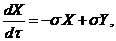
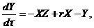
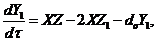
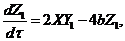
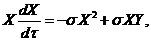
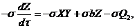
The revised three-dimensional Lorenz Model (3DLM) includes two general parameterization terms (e.g.,  and
and  ), as follows:
 (1)
(1)
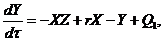 (2)
(2)
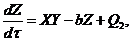 (3)
(3)
here,σandr are the Prandtl number the normalized Rayleigh number, respectively [1,2]. Note thatr is also known as the heating parameter.(X,Y,Z)represent the amplitudes of the solutions resolved by the Fourier modes of Lorenz [1]. In this study, the three modes in the 3DLM are referred to as primary modes.  and
and  represent the nonlinear feedback from small-scale processes, derived analytically from a higher-dimensional Lorenz model, e.g., 5DLM or 6DLM. As illustrated in Shen [2], nonlinear terms of the 3DLM, as well as 5DLM and 6DLM, come solely from the advection of temperature perturbations. Thus, only including additional nonlinear terms in Eqs. 2 and 3 is justifiable. Detailed procedures regarding the choices for
  and
and  using the 5DLM or 6DLM are provided below.
2.1 3DLM with parameterization using the 5DLM (3DLM-P5d)
In the following, determination of Q1 and Q2 using the 5DLM, which consists of the following equations [2], is discussed:
 (4)
(4)
 (5)
(5)
 (6)
(6)
 (7)
(7)
 (8)
(8)
here, both  and
and  are constants (
 and
and  ) and are defined in Shen (2014) and Shen (2015)[2,7]. As compared to
  and
and  ,
,  and
and  represent the amplitudes of temperature perturbation modes that are resolved using two additional Fourier modes with high wave-numbers [2,7]. The two modes are referred to as secondary temperature modes. As defined in the previous studies [2,7], the term “feedback” refers to the nonlinear processes that involve the secondary modes (i.e.,
 and/or
  ). Therefore, Eqs. (4-6) in the 5DLM can be viewed as a 3DLM with the feedback processes (i.e.,
 ) that result from the secondary modes. Physically, the term
  represents the nonlinear advection of secondary temperature mode that provides feedback to the primary temperature mode.
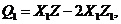
By comparing the revised 3DLM (i.e., Eqs. 1-3) with Eqs. (4-6) of 5DLM,  and
and  are first obtained. In Appendix A of Shen [2],
  was shown to be responsible for conversion of domain averaged potential energy between
  and
and  mode. Thus the negative nonlinear feedback of
  is also associated with the
  . Next, it is beneficial to express the secondary mode (i.e.,
 ) in terms of the primary modes (i.e.,
  ). To achieve this,
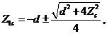
  is solved by assuming a steady-state solution for secondary modes in Eqs. (7-8), i.e.,
 and
and  , as follows:
 (9)
(9)
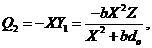 (10)
(10)
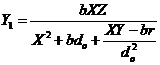
In Eq. (10), the nonlinear advection of secondary temperature mode is represented by the primary modes . With
  and
and  in Eq. 10, the revised 3DLM (Eqs. 1-3) is referred to as the 3DLM-P5d or 3DLMP5d. Note that Eq. (10) can be simplified, as follows: (1) When
  is small and
  is positive,
  where
where  is a tunable parameter. This type of parameterization with
  was first included in a revised 3DLM by Shen [2], who indicated that a larger
 is required for the onset of chaos. (2) When
  is large (i.e.,
  ),
),  and is the same as the dissipative term (
 ) in Eq. (6). Although it is challenging to linearize the revised 3DLM that includes a complicated nonlinear
  term(i.e., Eq. 10), the two simplified cases make it feasible to linearize Eq. (3) and to, thus, calculate Lyapunov vectors using the Gram-Schmidt reorthonormalization procedure discussed in Section 2.4. Additionally, these two simplified versions can be used to illustrate how changes in parameterizations may lead to different equilibrium-state solutions, as discussed below.
In Appendix A of Shen [2], domain-averaged kinetic energy ( ) and potential energy (
 ) are written, as follows:
 (11)
(11)
 (12)
(12)
Where . By multiplying Eqs. 1 and 2 by
  and
and  , respectively, one obtains:
 (13)
(13)
 (14)
(14)
Adding the two questions above yields:
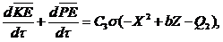 (15)
(15)
In Eq. (15), the nonlinear term ( ) associated with the primary modes is implicit and is internally responsible for energy conversion, while the nonlinear feedback term involving the secondary modes is represented by
  . The three terms on the right hand side represent energy sinks (or sources),
 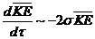 and
and  . As discussed,
  in Eq. (10), and
  plays a role similar to
  , which adds negative potential energy into the system (Eq. 12) and provides negative thermodynamic feedback. A steady-state solution is reached when the right hand side of Eq. (15) equals zero. The steady-state solution with
  is the critical point solution of the 3DLM (i.e.,
 ). With the general form of
  in Eq. 10, a steady-state solution appears when the primary modes (
 ) are replaced by the analytical solutions of the critical points in the 5DLM (Eqs. 19a-c of Shen, 2014), written, as follows:
 (16a)
(16a)
 (16b)
(16b)
 (16c)
(16c)
Eq. (16) suggests that steady-state solutions in the 3DLMP5d are the same as those of the 5DLM. Since parameterization of nonlinear feedback is based on the assumption of steady-state solutions for the secondary modes in the 5DLM, the result is anticipated. As discussed earlier, the parameterized term ( ) is dominated by
  with
with  when
when  is relatively small and is dominated by
  when
when  is relatively large. The two simplified cases lead to the following different steady-state solutions: 1)
  and 2)
  , respectively. Note that
  has the same form as Eq. (16a) for the 3DLM, the revised 3DLMs, and the 5DLM. Therefore, by choosing a different
  , we can change the equilibrium-state solutions for the revised 3DLM (Eqs. 1-3) (e.g., from the fixed-point solutions of the 3DLM, when
  , to fixed-point solutions of the 5DLM, when
  is described by Eq. 10). Although proper selection of
  (=1/2) in the the first simplified case may lead to the same equilibrium-state solutions as those of the second simplified case, their time-varying solutions are still different. In fact, when
  is small as compared to
  in Eq. (10), this condition poses an upper bound on
  (or
(or  ) as a result of
 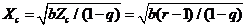 . The parameterized term (
 ) emulates the nonlinear feedback associated with the nonlinear advection of temperature and dissipative processes due to the secondary modes. Thus, any simplifications in
  indicate changes in the nonlinear advection and/or dissipation. The above discussions suggest the dependence for both transient and stead-state solutions on the detailed implementation of a parameterization, including nonlinear advection and/or dissipative processes. Further illustration with numerical results are provided in Figure 4 and discussed in Section 3.
2.2 3DLM with parameterization using the 6DLM (3DLM-P6d)
To emulate the nonlinear feedback associated with the secondary modes, the above approach assumes a steady state solution for the secondary modes and, thus, represents the secondary modes in terms of primary modes. To further assure the validity of the approach, a test is performed with the 6DLM. Incremental changes in the number of Fourier modes from the 3DLM, to the 5DLM and 6DLM can help trace the individual and/or collective impact on solution stability. While the secondary temperature modes ( and
and  ) of the 5DLM, as well as the 6DLM, introduce additional nonlinear and dissipative terms, which, in turn, provide negative nonlinear feedback, the secondary streamfunction mode (
 ) of the 6DLM (Eqs. 4-5 of Shen (2015)[7]) introduces additional nonlinear terms and adds a heating term. Therefore, these LMs were used to examine the competing impact between an additional heating term and the negative nonlinear feedback [7]. Research has indicated the following: 1) negative nonlinear feedback in association with the secondary temperature modes plays a dominant role in providing feedback for improving the solution stability of the 6DLM; 2) the additional heating term in association with the secondary streamfunction mode may destabilize the solution, but its impact is much smaller than that of the negative nonlinear feedback. Thus, the 6DLM has a comparable but slightly smaller
  (
( ) for the onset of chaos, as compared to the 5DLM with
  (Table 1). The 5DLM and 6DLM collectively suggest different roles for small-scale processes (i.e., stabilization vs. destabilization).
Following the aforementioned procedures in Section 2.1, the revised 3DLM (Eqs. 1-3) is compared with the 6DLM (e.g., Eqs. 8-10 of Shen, 2015[7]) to obtain the following:
 (17)
(17)
 (18)
(18)
Using Eqs. (11-13) of Shen (2015)[7], steady state solutions for  ,
,  and
and  are solved and and expressed in terms of (
 ):
):
 (19)
(19)
 (20)
(20)
 (21)
(21)
Now, both  and
and  in Eqs. (17-21) are functions of the primary modes (
 ). The revised 3DLM (Eqs. 1-3) using Eqs. (17-21) is referred to as the 3DLM-P6d or 3DLMP6d. In Section 2.4, we discuss numerical approaches for the calculation and analysis of solutions in both 3DLMP5d and 3DLMP6d.
Dissipation vs. Numerical Smoothing
The above discussions emphasize the role of negative nonlinear thermodynamic feedback in improving solution stability. The relationship of the nonlinear feedback to the additional nonlinear terms (i.e., ) and the dissipative term (i.e.,
 ) was discussed in Shen (2014) [2]. An important question to be answered is how these processes may be identified in real world models such as climate models and/or weather models [13-15]. While it takes a significant effort to thoroughly address this question, an initial attempt is made in the following discussion. The nonlinear term,
 , representing the horizontal and vertical advection of temperature, is commonly included in numerical models (explicitly or implicitly). While the dissipative term may be physically interpreted as an eddy dissipative process, it can be numerically linked to an averaging operator, as discussed below. For example, the dissipative term
  can be simplified, as follows:
 (22a)
(22a)
and the rate of change in  can be approximated by
 (22b)
(22b)
Here,  and
and  represent a grid spacing and time interval, respectively. By choosing
  , we have
 (23)
(23)
The above, which is approximated from the linear thermodynamic equation with the dissipative term (i.e., ), qualitatively suggests that the averaging operator plays a role numerically similar to the Laplacian operator (
 ) in contributing to dissipative processes.
Numerical approaches
Using the 4th order Runge-Kutta scheme, the original and revised Lorenz models are integrated forward in time. The value of the heating parameter,  , is varied, while other parameters, including
  ,
,  , and
, and  , are held constant. The dependence of solution’s stability on
  was examined using the 3DLM, 5DLM, 6DLM and a revised 3DLM with
  and
and  [2,7]. Below, the ensemble Lyapunov exponents are first discussed then followed by time-dependent solutions obtained from the 5DLM, 3DLMP5d, and 3DLMP6d. Numerical approaches, as discussed by Shen [2], are also briefly summarized.
For the time-dependent solutions, the initial conditions are, as follows:
 (24)
(24)
The dimensionless time interval ( ) is
) is  . The total number of time steps (
 ) is 500,000. To quantitatively evaluate whether or not the system is chaotic, we calculate the Lyapunov exponent (LE), a measure of the average separation speed of nearby trajectories on the critical point [16-25]. In Shen [2], the two methods implemented and tested are the trajectory separation (TS) method [23]and the Gram-Schmidt reorthonormalization (GSR) procedure[17,21]. Using given initial conditions (ICs) and a set of parameters in the LMs, the TS scheme calculates the largest LE while the GSR scheme produces "n" LEs. Here, "n" is the dimension of the 5D or 6DLM. Obtaining the n LEs using the GSR scheme requires the derivation of the so-called variational equation. Calculations are conducted with
  and
and  , yielding
  . To minimize dependence on the ICs, 10,000 ensemble (
 ) runs with the same model configurations but different ICs are performed, and an ensemble averaged LE (eLE) is obtained from the average of the 10,000 LEs. A large
  and
and  are used to understand the long-term average behavior of the solutions in the LMs. The eLEs calculations of the 3DLM, 5DLM and 6DLM, obtained using the two methods above, were previously discussed and compared in Shen [2,7]. A calculation of the Kaplana & Yorke fractal dimension [26]using the (three) leading eLEs from the GSR method was provided in Appendix A of Shen [7], as an additional verification. The results of the 3DLM, obtained using both methods, are presented for a comparison. Only the TS method is applied in the 3DLMP5d and 3DLMP6d because both models introduce complicated nonlinear terms, making it difficult to derive the variational equation for the GSR scheme.
For stable solutions, as shown by numerical solutions to be discussed in Section 3, the 3DLMP5d and 3DLMP6d produce the same steady-state solutions as those in the 5DLM and 6DLM, respectively. The result is expected due to the assumption of the parameterization, as discussed in Sections 2.1 and 2.2. As nonlinear feedback processes are emulated with diagnostic equations in the revised 3DLMs and as nonlinear feedback processes are resolved by prognostic equations in the 5DLM and 6DLM, the revised 3DLMs are unable to accurately depict the evolution of transient solutions in both phases and amplitudes prior to the steady state, as compared to solutions in the 5DLM or 6DLM. Therefore, using a different methodology for comparing the time-varying solutions of the revised 3DLMs and the corresponding high-dimensional LMs is important.
A common practice is to compare the time averaged quantities of two fields in place of a direct point-to-point comparison. However, it is not trivial to determine a time scale for averaging, in particular when a solution evolves at multiple scales. Therefore, to achieve the goal of comparing solutions from different LMs, the trend mode, defined as the non-oscillatory component of the solution, is calculated and compared. The core technology for this calculation is the empirical mode decomposition (EMD) [27,28]. The EMD, as first developed by Huang et al.[27], extracts a finite number (N) of the oscillatory intrinsic mode functions (IMFs) from the local extrema of the data. The residual, which represents the difference between the raw data and a sum of N IMFs, is called the trend mode, which is non-oscillatory. The ensemble EMD (EEMD) method was proposed to effectively resolve the issue of mode mixing in the EMD [28]. Although the method is promising, it requires tremendous computing resources, as computational resources are linearly proportional to the number of ensemble trials. To reduce the time to obtain solutions, we have developed a parallel version of EEMD (PEEMD) with a three-level parallelism using message-passing interface (MPI) tasks for the first two levels and with OpenMP threads in the third level [29-31]. The PEEMD leads to a parallel speedup of 720 using 200 eight-core processors, and is used to calculate the trend modes in Figure 4c.
Numerical Results
Figure 1 provides ensemble Lyapunov exponents (eLEs) as a function of the normalized Rayleigh parameter ( ) for the 3DLM, 5DLM, and revised 3DLMs (i.e., 3DLMP5d and 3DLMP6d). Table 1 summaries the critical value (
 ) for the onset of chaos in these models. As first indicated in Shen [2], the 5DLM requires a larger
  for the onset of chaos than the 3DLM. The critical value (
 ) of the 5DLM is 42.9 while the
  of the 3DLM is 24.74. It was shown that the negative nonlinear feedback via the
  term can help suppress chaotic responses.
  is present in the 5DLM but not in the 3DLM. Since the 3DLMP5d includes the impact of
  by assuming a steady-state solution for
  and
and  in Eqs. (7-8), the critical value (
 ) is expected to be comparable to that of the 5DLM and larger than that of the 3DLM, as shown in Figure 1 and Table 1. Interestingly, the
  of the 3DLMP5d is 52.1, which is larger than that of the 5DLM. The result suggests that the solution of 3DLMP5d is less chaotic than that of the 5DLM, and that the transient evolution of small-scale processes by the secondary modes, which appear associated with nonzero
  and
and  in the 5DLM, may destabilize the solution of the 5DLM, as further discussed using Figure 4.
The 6DLM was derived to illustrate the competing impact of an additional heating term and negative nonlinear feedback [7]. It was shown that the negative nonlinear feedback plays a dominant role in providing feedback, and that the 6DLM has a comparable but slightly smaller  (41.1) as compared to the 5DLM. The negative nonlinear feedback and the impact of an additional heating term in the 6DLM are emulated in the 3DLMP6d using steady-state solutions for the secondary modes. Therefore, the 3DLMP6d with two parameterized terms is used to ensure the validity of the nonlinear thermodynamic parameterization. In Figure 1 and Table 1, the
  of the 3DLMP6d is 51.4, which is comparable, but slightly smaller, than that of the 3DLMP5d (
 ). Similarly, the 6DLM has a smaller
  than that of the 5DLM. Figure 2 displays Y-Z plots with
  from the 3DLM, 5DLM, 3DLMP5d, and 3DLMP6d, indicating a chaotic solution for the 3DLM but stable solutions for the rest of the LMs.
To illustrate how the revised 3DLMs, as well as the 5DLM, reach a steady-state solution with  , we analyze the terms on the right hand side of Eq. (6), including
  ,
,  , and
, and  . Figure 3 indicates that the first two terms are balanced with the
  in order to have a steady-state solution. When the feedback of
  is added into the 3DLMP5d, solutions for the
  and
and  (Figure 3b) are comparable to those of the 5DLM, indicating that
  and
and  are balanced with
  in the 3DLMP5d. The corresponding solutions of the 3DLMP6 (Figure 3c) are also comparable to those of the 5DLM and 3DLMP5, indicating the validity of the approach in determining and emulating the nonlinear feedback using the 6DLM.
A more detailed comparison is provided in Figure 4 where the transient solutions for  and
and  from the 5DLM, 3DLMP5 and 3DLMP6 are examined. As indicated in panels (a)-(b), all of the solutions eventually become steady, while the solution of the 5DLM displays a smaller decay rate. In the zoomed-in view (Figure 4c), the oscillatory solution of 5DLM displays larger amplitudes as compared to those of the 3DLMP5 and 3DLMP6. A comparison of the solutions obtained from the 3DLMP5d and 3DLMP6d indicates that the latter, with an additional term (i.e.,
 ), produces a solution with a comparable amplitude but a different phase, as compared to the former solution. The result is consistent with that of Shen [7]in that the positive feedback associated with the secondary streamfunction mode is small as compared to the negative feedback largely associated with the secondary temperature modes. To compare the evolution of different solutions, Figure 4c displays the trend mode of the solutions at the early stage (i.e.,
 ). While transient solutions from the revised 3DLMs with parameterizations (3DLMP5 and 3DLMP6) produce large differences in both phases and amplitudes, their trend modes are very close to that of the 5DLM. The result implies that the revised 3DLMs with parameterizations, which are emulated from the feedback of secondary modes, can produce comparable time averaged solutions as compared to the 5DLM or 6DLM, and lead to the same steady-state solutions when
  is smaller than the
  of the 5DLM (or 6DLM).
The above discussions demonstrate that nonlinear feedback (i.e.,  ) in the 5DLM can be analytically expressed in terms of original Fourier modes within the 3DLM, and that feedbacks can be emulated by introducing an additional term (i.e.,
  ) into the 3DLM. The term, which emulates the collective impact of the horizontal advection of temperature perturbation and dissipations associated with the high-wavenumber modes, can be analytically determined by solving for a steady-state solution for the high-wavenumber modes within the high-dimensional LM (e.g., 5DLM), as discussed in section 2.1. Using this approach, the revised 3DLM is viewed as the 3DLM with nonlinear feedback parameterized by the additional term. This approach is referred to as the parameterization of nonlinear thermodynamic feedback.
Concluding Remarks
The sensitive dependence of numerical solutions on initial conditions (ICs), appearing in the 3DLM when the normalized Rayleigh parameter ( ) exceeds a critical value (
 ), is known as chaos or butterfly effect of the first kind. Although chaotic solutions are associated with the inclusion of nonlinearity (as indicated in a comparison between the nonlinear 3DLM and linearized 3DLM), increased degrees of nonlinearity in higher-dimensional Lorenz models can improve system stability, since both the 5DLM and 6DLM require a larger
  for the onset of chaos [2,7] (Table 1). In this study, we proposed the revised Lorenz model with only one parameterized term (i.e., 3DLMP5d) that can produce more stable solutions as compared to the 3DLM. The new term is added to emulate the nonlinear thermodynamic feedback that was first identified in the 5DLM. By analyzing the nonlinear term,
 , using five modes (for the 5DLM), the negative nonlinear feedback of the secondary modes can be mathematically represented by the
  term in Eq. (6). Using the term
  , we demonstrated how to incorporate the negative nonlinear feedback into the revised 3DLM without using additional prognostic equations, based on the following: (1) We added a parameterized term
  , which is equal to
  , into a revised 3DLM. (2) We obtained steady-state solutions for the secondary modes (e.g.,
  and
and  in the 5DLM) and expressed
  in terms of the primary modes (
 ). Therefore, the nonlinear feedback processes are emulated using diagnostic equations in the revised 3DLMP5d, while they are explicitly resolved by prognostic equations in the 5DLM. A different simplification of the parameterized
  was found to lead to a different equilibrium state solution, indicating the dependence of the equilibrium state solution on the changes in nonlinear advection associated with the secondary or high-wavenumber modes. For example, the critical point
  in the revised 3DLM using a different
  can be
  ,
,  ,
,  , or
, or  when
when  equals
  ,
,  ,
,  , or
, or  (Eq. 10), respectively.
When the 6DLM is used to emulate the nonlinear feedback, two parameterized terms are added to a revised 3DLM using similar procedures, as discussed in Section 2.2. The revised 3DLM, with the parameterized term(s) that is (are) emulated using the 5DLM (6DLM), is referred as to the 3DLMP5d (3DLMP6d). Table 1 summarizes critical values for the onset of chaos in the 3DLMP5d, 3DLMP6d, 3DLM, 5DLM, and 6DLM. For chaotic solutions, the  of the 3DLMP5d is
  , which is larger than that of the 3DLM (
 ). The value is comparable to but larger than the
  of the corresponding 5DLM (
 ). Similar characteristics are observed when comparing the 3DLMP6d and 6DLM, which yield
  values of 51.4 and 41.1, respectively. The above features suggest that the stability of the 3DMLP5d (3DLMP6d) is overestimated between
  (
( ), as compared to the 5DLM (or 6DLM). For stable solutions, the revised 3DLM produces the same steady-state (equilibrium-state) solutions as those in the 5DLM (or 6DLM) when parameters are set to be the same in the models (e.g.,
  ). Although the revised 3DLM (3DLMP5d or 3DLMP6d) is unable to accurately represent the evolution of transient solutions in both amplitudes and phases, as compared to the 5DLM, the trend mode of its transient solution is comparable to that of the 5DLM. The trend mode is determined using the newly developed parallel ensemble empirical mode decomposition (PEEMD) method. The characteristics of solutions such as overestimated stability, lack of detailed evolution, and a comparable trend mode are often found in the comparisons of coarse-resolution climate model and fine-resolution climate (or weather) model simulations.
This study and previous studies [2,7] have discussed the role of negative nonlinear thermodynamic feedback in improving solution stability and showed its relationship to the additional nonlinear terms (i.e., ) and the dissipative term (i.e.,
  ). A nonlinear feedback loop consists of a pair of downscale and upscale transfer processes via the Jacobian term[2], and can be continuously extended as long as new modes can be continuously generated. The extended nonlinear feedback loop may further stabilize or destabilize system solutions. The mathematical analysis provided in section 2.3 suggests that an averaging operator may contribute to dissipative processes, which play a role numerically similar to the Laplacian operator (
 ). As nonlinear advection terms and averaging operators are often included in climate models, we hypothesize that the nonlinear feedback of numerical averaging/smoothing may suppress chaotic responses, leading to more stable solutions. This hypothesis will be examined using higher-dimensional Lorenz models and climate/weather models with the TS method in a future study. As numerical averaging may impact the phase and amplitude of transient solutions, posing a challenge for verifying time-varying numerical solutions against observations (or, comparing the transient solution obtained from a low- and high-dimensional models), an alternative method such as the PEEMD for comparing their trend modes is required. Detailed analyses and comparisons of the different Lorenz models and their application to climate model simulations are currently being planned.
Acknowledgments
I thank Drs. R. Pielke Sr., Y.-L. Lin, R. Anthes, and X. Zeng for valuable comments and encouragement, and Dr. Y.-L. Wu for proofreading this manuscript. I am grateful for support from the College of Science at San Diego State University, the NASA Advanced Information System Technology (AIST) program of the Earth Science Technology Office (ESTO). Resources supporting this work were provided by the NASA High-End Computing (HEC) Program through the NASA Advanced Supercomputing division at Ames Research Center.
References
- Lorenz E (1963) Deterministic nonperiodic flow. J Atmos Sci 20: 130-141.
- Shen BW (2014) Nonlinear Feedback in a Five-dimensional Lorenz Model. J Atmos Sci 71: 1701-1723.
- Gleick J (1987) Chaos: Making a New Science. New York. Penguin. 360pp.
- Pielke R (2008) The Real Butterfly Effect, 477.
- Anthes R (2011) "Turning the tables on chaos: Is the atmosphere more predictable than we assume?" UCAR Magazine, spring/summer.
- Strogatz SH (2015) Nonlinear Dynamics And Chaos: With Applications To Physics, Biology, Chemistry, And Engineering.
- Shen BW (2015) Nonlinear Feedback in a Six-dimensional Lorenz Model. Impact of an additional heating term. Nonlin Processes Geophys Discuss 2: 475-512.
- Lorenz E (1972) "Predictability: does the flap of a butterfly’s wings in Brazil set off a tornado in Texas?" Talk presented Dec. 29, AAAS Section on Environmental Sciences, New Approaches to Global Weather: GARP. Boston, Mass.
- Curry JH (1978) Generalized Lorenz Systems. Commun Math Phys 60: 193-204.
- Curry JH, Herring JR, Loncaric J, Orszag SA (1984) Order and disorder in two- and three-dimensional Benard convection. J Fluid Mech147: 1-38.
- Musielak ZE, Musielak DE, Kennamer KS (2005) The onset of chaos in nonlinear dynamical systems determined with a new fractal technique. Fractals 13: 19-31.
- Roy D, Musielak ZE (2007a) Generalized Lorenz models and their routes to chaos. I. energy-conserving vertical mode truncations. Chaos, solitons and Fractals 32: 1038-1052.
2021 Copyright OAT. All rights reserv
- Shen BW, Atlas R, Reale O, Lin SJ, Chern JD, et al. (2006) Hurricane forecasts with a global mesoscale-resolving model: preliminary results with hurricane Katrina (2005). Geophys Res Lett 33.
- Shen BW, Tao WK, Lin YL, Laing A (2012a) Genesis of Twin Tropical Cyclones as Revealed by a Global Mesoscale Model: The Role of Mixed Rossby Gravity Waves. J Geophys Res 117: D13114.
- Shen BW, DeMaria M, Li JLF, Cheung S (2013a) Genesis of Hurricane Sandy (2012) Simulated with a Global Mesoscale Model. Geophys Res Lett 40.
- Froyland J, Alfsen KH (1984) Lyapunov-exponent spectra for the Lorenz model. Physical Review A 29: 2928-2931.
- Wolf A, Swift JB, Swinney HL, Vastano JA (1985) Determining Lyapunov Exponents from a Time Series. Physica 16D: 285-317.
- Nese JM (1989) Quantifying local predictability in phase space. Physica 35D: 237-250.
- Zeng X, Eykholt R, Pielke RA (1991) Estimating the Lyapunov-exponent spectrum from short time series of low precision. Phys Rev Lett 66: 3229-3232. [Crossref]
- Eckhardt B, Yao D (1993) Local Lyapunov exponents in chaotic systems. Physica D 65: 100-108.
- Christiansen F, Rugh H (1997) Computing Lyapunov Spectra with Continuous Gram-Schmid Orthonormalization. Nonlinearity 10: 1063-1072.
- Kazantsev E (1999) Local Lyapunov exponents of the quasi-geostrophic ocean dynamics. Applied Mathematics and Computation104: 217-257.
- Sprott JC (2003) Chaos and Time-Series Analysis. Oxford University Press. 528pp. The numerical method is briefly discussed on http://sprott.physics.wisc.edu/chaos/lyapexp.htm.
- Ding RO, Li JP (2007) Nonlinear finite-time Lyapunov exponent and predictability. Phys Lett 354A: 396-400.
- Li J, Ding R (2011) Temporal-Spatial Distribution of Atmospheric Predictability Limit by Local Dynamical Analogs. Mon Wea Rev 139: 3265-3283.
- Kaplan JL, YorkeJA (1979) Chaotic behavior of multidimensional difference equations. In: Functional differential equations and the approximations of fixed points, Peitgen HO, Walther HO (Eds.), Lect. Notes in Math. 730, Springer-Verlag, New York, 228-37.
- Huang NE, Shen Z, Long SR, Wu MC, Shih SH, et al. (1998) The empirical mode decomposition and the Hilbert spectrum for nonlinear and non-stationary time series analysis. Proc R Soc Lond A 454: 903-995.
- Wu Z, Huang NE (2009) Ensemble Empirical Mode Decomposition: a noise-assisted data analysis method. Advances in Adaptive Data Analysis 1: 1-41.
- Shen BW, Wu Z, Cheung S(2012b) Analysis of Tropical Cyclones and Tropical Waves using the Parallel Ensemble Empirical Model Decomposition (EEMD) Method. AGU 2012 Fall Meeting, San Francisco, December 03-07, 2012.
- Shen BW, Cheung S, Li JLF, Wu YL (2013b) Analyzing Tropical Waves using the Parallel Ensemble Empirical Model Decomposition (PEEMD) Method: Preliminary Results with Hurricane Sandy (2012), NASA ESTO Showcase by Earthzine magazine. posted December 2, 2013.
- Cheung S, Shen BW, Mehrotra P, Li JLF (2013) Parallelization of the Ensemble Empirical Model Decomposition (PEEMD) Method on Multi- and Many-core Processors. AGU 2013 Fall Meeting, San Francisco, December 9-13.