Oil sand is a composite material of quartz aggregates, bitumen, water, and air void in which the bitumen exhibits a time and temperature dependent behavior under loading. The soil skeleton (quartz aggregates) comprises dense, highly incompressible, and uncemented fine interlocked grains exhibiting low in-situ void ratio, and high shear strengths and dilatancy under low normal stresses. In this work, a 2D discrete element method (DEM) is developed to model the viscoelastic response of an oil sand formation. A digital sample of the oil sand with varying particle shapes and sizes were built using the discrete element software PFC2D. The oil sand microstructure was captured from a scanning electron microscope image of a 14.5% bitumen content Athabasca oil sand. The micromechanical approach is based on discretizing the oil sands microstructure and modeling particle interactions (contacts) of its constituents at microscale. The quartz aggregates, water, and bitumen included in the digital samples were modeled using different contact models. Rheological data for the bitumen was obtained from a stress/strain controlled rheometer equipped with a parallel plate. This data was used to calibrate the parameters of the viscoelastic contact models among the different material phases. The resulting parameters of Burger’s model were used to simulate the micromechanical behavior of the material. A 2D DEM model with two temperatures and three loading frequencies subjected to a constant amplitude sinusoidal compression tests was simulated. The results of the study show a good agreement between the model prediction and the measured dynamic modulus and phase angle. This indicates that the linear viscoelastic DEM model developed is capable of simulating time-dependent behavior of oil sands material. Additionally, the effect of rate of loading and temperature on the deformational mechanics of the material was evident in the dynamic modulus determination.
Oil sand is a dense granular material whose two main physical compositions are quartz grains and large quantities of interstitial bitumen, as shown in Figure 1. The pore spaces of oil sands are also filled with dissolved gasses and water [1-3]. The water is a thin film (~10 nm) that surrounds the quartz grains (about 99% water-wet) [4]. The connate water fills 10-15% of the pore spaces and the remaining is occupied by bitumen [1].
Figure 1(b) reveals that the grain-grain contact in oil sand formations exhibit mainly long and concavo-convex contacts. This structure is known as interpenetrative and is responsible for both the low void ratio and high shear strength [5]. Additionally, a large number of contacts per grain are formed because of the dense structure and consequently the formation undergoes high dilation at low normal stresses. The oil sand formations are mined for crude oil production in Northern Alberta, Canada. Surface mining methods, using ultra-class mining equipment such as the P&H 4100 BOSS ERS and the CAT 797 dump trucks are used for bulk excavation of the overburden, providing access to the oil-rich formation. These equipment units impose varying magnitudes of static and dynamic loading in both the horizontal and vertical directions to the ground during excavation. This has led to equipment sinkage/rutting, lower frame fatigue failure [6], and wear, and tear of crawler shoes [7].
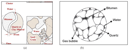
Figure 1. Microstructural section of Athabasca oil sand: (a) In-situ structure of oil-rich quartzose oil sand [1]; (b) Idealized section of in situ oil sand [5]
Soils in general exhibit both elastic (recoverable) and plastic (permanent deformation) behavior under loading. However, oil sands exhibit viscous flow in addition to elastic and plastic behavior under loading. The internal structure of the oil sands shows a discrete behavior as relative positions of quartz particles are changed under loading. The overall macromechanical behavior of the formation is determined by the interaction between its constituents because of its discrete structure and multiphase composition. Thus, a micromechanical model is required to comprehensively simulate the heterogeneous, nonlinear, and anisotropic behavior of the formation.
The objective of this paper is to model the micromechanical and microstructural behavior of oil sands formation as a multiphase material using the DEM technique to understand its complete rheological behavior from elastic to viscoelastic cases. The study also performs the determination of macroscale material properties and the calibration of the microscale model parameters. In this study, macroscale material properties of bitumen [32] and quartz aggregates [13] are measured in the laboratory. A set of equations developed by [25] were employed to express the relationship between the microscale DEM model parameters and the macroscale material properties. A nonlinear optimization technique was applied to fit the Burger’s viscoelastic contact model using the dynamic modulus laboratory test at different loading rate and temperature.
Over the last three decades, the stress/strain behavior of oil sands has been studied using mainly experimental, analytical, and numerical approaches. Many researchers have used experimental methods to (i) develop a constitutive model to predict the effective stress/strain behavior of drained and recompacted oil sands [8-10], (ii) characterize the shear strength and permanent deformation behavior [3,11-13], and (iii) study the microscopic structure [1,5]. The outcome of these testing procedures predicts the macromechanical stress/strain response of the formation. Additionally, the results of the studies show that quartz grain surface rugosity and grain angularity are functions for the higher residual strength of the oil sand material.
Within the last two decades, the use of numerical methods to model and simulate the behavior of particulate media has gained popularity as a tool for fundamental studies [14-16]. Two numerical methods commonly utilized are the finite element method (FEM) and DEM. Numerical approaches using FEM produce some advantages over the analytical and experimental approaches [17-21]. Material models developed from these methods are either micromechanical or macromechanical in nature. In macromechanical approaches, a constitutive model is used to represent the global material behavior that considers the material as a continuum. On the other hand, the micromechanical approach is based on discretizing the composite microstructure and modeling the material properties of its constituents [22]. Recently, Gbadam and Frimpong [17], and Brown and Frimpong [18] used FEM to simulate the nonlinear mechanical response of geomaterials and oil sands in formation-tool interactions. FEM is based on continuum mechanics, which lacks the ability to handle large strains and discontinuous strain fields. Hence, model slippage between the aggregate particles, which has been cited as one of the most important mechanisms resulting in permanent deformation or rutting [23], cannot be addressed using FEM. Such limitation can be addressed by an alternative DEM approach.
Over the past decade, several researchers have used DEM to simulate discontinuous materials with some success. Current research efforts indicate little or no application of DEM for modeling a composite material, such as oil sands. However, DEM has been used to model the heterogeneous multiphase material of asphalt mixtures [15,24], and a number of researchers have developed micromechanical models with the DEM [25]. The mechanical behaviors of asphalt mixtures are simulated with an elastic model [26-28], a viscoelastic model [15,25,29], and a cohesive model [30]. The elastic models are time-independent, and thus, not suitable to simulate a time-dependent material like the oil sands. The viscoelastic behavior of asphalt mastic is represented with Burger’s model. The Burger’s model is a four-component model consisting of a Maxwell element and Kelvin element in series, where the normal and shear stiffness changes with time. Under constant stress, Burger’s model can simulate instantaneous strain, viscoelastic response, instantaneous recovery, and permanent strain [15].
In oil sand modeling and simulation, little or no work has been done to formulate its micromechanical and microstructural behavior based on DEM. Recently, Tannant and Wang [31] conducted a numerical (using DEM) and experimental study of wedge penetration into compacted oil sand to measure the force required to push the steel wedge into oil sand formations. The force computed using the numerical model was about four to six times higher than that measured experimentally. This discrepancy between the model and laboratory test may be due to simplification of the DEM model.
Discrete element method
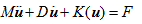
The DEM technique is a numerical method introduced by [14] for rock mechanics analysis and then extended by [33] for soil as an alternative to continuum modeling of particulate media. In continuum mechanics, the soil is assumed to behave as a continuous material. The study does not consider the relative movement and rotation of soil grains necessary to understand the micro-level soil behavior. Newton’s second law and finite difference scheme are used to study the mechanical interactions between a large collection of independent and varying discrete particles with rigid or deformable bodies. As the particles and bodies (walls) interact with each other, creating contacts, a force-displacement law (usually termed contact model) is used to update the contact forces and moment arising from the relative motion at each contact. The translational and rotational motion of each particle is calculated from the contact forces and moment using Newton’s second law. The overall governing equation of motion for the dynamic analysis of the DEM system is expressed as Equation (1):
 (1)
(1)
 are the linear and rotational acceleration, velocity, and displacement vectors, respectively; M is mass (including rotational inertia); D is damping; K is internal restoring force; and F is the external force (including moments).
The dynamics (translational and rotational motion) of the particle i with mass mi and moment of inertia Ii are governed by the Newton and Euler terms in Equation (2) and (3) [34,35]:
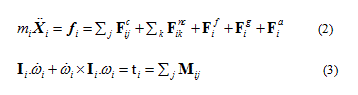
 are the translational and angular accelerations of particle i, respectively;
 is the angular velocity of particle
  are the sum of forces and torques acting on particle i respectively
  ; and are the contact force and torque acting on particle i by particle j or rigid/flexible boundary;
  is the non-contact force acting on particle i by particle k (example of non-contact force would be capillary force from a wet media); and
  are the fluid, gravitational, and applied force on particle i. The soft contact approach is used where the particles are assumed to be rigid but allows overlap at the contact points. The contact force is related to the magnitude of the overlap and is computed using a force-displacement law (contact model). The development and implementation of a realistic contact model at the micro level is the heart of the particle-based simulation. The simplest contact model that can be selected consists of a spring and dashpot connected in series, where the contact force is computed in equations (4) and (5) [36]:
 is force in the normal direction of the plane of the contact,
  is the overlap between the particles in the normal direction,
  is the tangential force, and
  is the relative displacement in the tangential direction. Figure 2 illustrates the typical forces and torques at particle contacts.
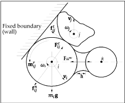
Figure 2. Forces acting on particle (ball) i with particle (clump) j and non-contacting particle K [34].
Local constitutive models or contact models are used to characterize the different material behavior at the macro level by calculating the contact forces and torques. A full description of the DEM algorithm is published in [14,33,37].
Design of PFC model for oil sands
In this study, the oil sand numerical specimen was constructed with a given number of clumps generated with pore spaces to match the actual particle size distribution (PSD). Figure 3 shows the PSDs of the real sample and the corresponding generated numerical model in PFC2D. Due to high computational expense, the fine particles (i.e., passing #200 sieve or <0.075 mm) were not included in the PFC model.
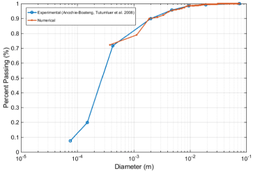
Figure 3. Particle size distribution of oil sand sample.
Oil sands with water and bitumen content of 2.2% and 14.5%, respectively, were modeled and simulated. The bitumen was microscopically represented by two sets of Burger’s element model in the normal and the tangential direction at each contact. The water phase is not modeled explicitly but is represented by a pendular liquid bridge that forms between the contacting particles. To duplicate the microstructure of the formation (including aggregates shapes and sizes, the spatial distribution of bitumen, and void spaces), a digital sample of a thin section was delineated to categorize the various phases as shown in Figure 4.
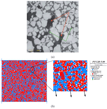
Figure 4. Internal structure of oil sand: (a) CT scan image [38]; (b) Numerical sample.
Three types of contacts that represent three different interactions within the sample are illustrated in Figure 5. The three corresponding contact models are associated with each contact to characterize the overall constitutive behavior of the oil sand material. The elastic linear model was defined at contacts between boundary walls and adjacent particles. The spring elements with stiffness  were used for the contact interactions between adjacent particles and boundary walls.
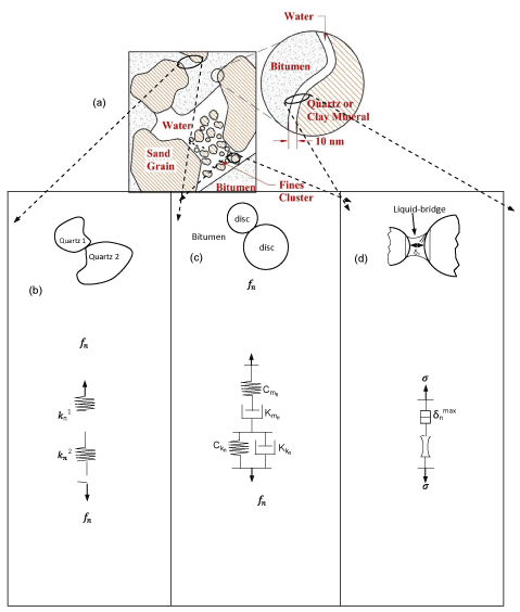
Figure 5. Particle contacts and corresponding force-displacement models of oil sand in the normal direction: (a) Microstructure (Takamura, 1982); (b) Adjacent aggregates (quartz-quartz contact); (c) Within bitumen (disc-disc contacts); (d) Between aggregate, water, and bitumen.
A clump with a mass, centroid position, and inertia tensor connected by elastic elements (springs and dashpots) in the normal and tangential directions at each contact is used to model the quartz. The interactions within a bitumen or between particle-bitumen are modeled with Burger’s element in the normal and shear directions. Burger’s element model, shown in Figure 6, provides a Kelvin model (linear spring and dashpot connected in parallel) acting in series with a Maxwell model (linear spring and dashpot connected in series) [39].
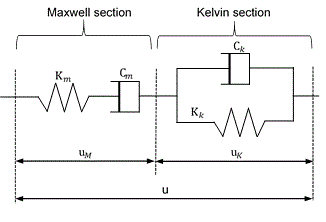
Figure 6. Burger’s model.
Equations (6), (7), and (8) express the constitutive behaviors of a Burger model at a contact [25,39]:
 are contact forces in normal and shear directions, respectively, at a contact;
  are the relative displacements in the normal and shear directions at a contact, respectively;
  are normal and shear displacement of the Kelvin model element;
  are normal and shear displacements of the spring element of the Maxwell model;
  are normal and shear displacements of the dashpot element of the Maxwell model;
  and are stiffness of spring elements; and
  are viscosities of dashpot elements.
Using Equations (6)-(8), the second-order differential equation for contact force, f is given by Equation (9):
The contact relations (model parameters) between two microscopic particles are directly defined at the contacts when using Burger’s contact model. These model parameters cannot be determined directly from the experimental results. Therefore, a macroscale Burger’s model, as shown in Figure 7, is correlated to an experimental dynamic shear modulus and phase angle data.
The response of Burger’s model subjected to either dynamic stress or strain is characterized using the complex compliance or the complex modulus and its constitutive equations can be derived as follows: The complex compliance is given in Equation (10):
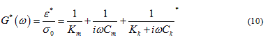
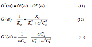
 are the stress and strain at time equal to zero and is the radial frequency. Equation (11) is normally decomposed into real and imaginary portions as shown in Equation (12-14) [40].
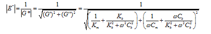
The dynamic complex modulus  is the reciprocal of the complex compliance, which is given in Equation (15):
 14
14
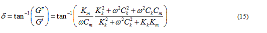
The phase angle  can be expressed as in Equation (16):
Once the macroscopic parameters are obtained, the microscopic input data were determined using the set of equations developed by Liu, et al. [25].
To obtain the macroscopic parameters, a nonlinear fitting technique must be utilized to fit the nonlinear experimental data from dynamic shear rheometer measurements. To fit the Burger’s model parameters, Papagiannakis, et al. [41] evaluated several objective functions and found that the objective function proposed by Baumgaertel and Winter [42], as given in Equation (10), provided the best fit. Two rheological measurements were fitted simultaneously, namely the storage and the loss shear moduli. The fitting procedure was based on minimizing an objective function (Equation 17) that is equal to the sum of squares of errors in predicting the storage and shear loss moduli over the available range of testing frequencies. Recently, this method was implemented to fit Burger model parameters for asphalt mastic [22,43].

 are respectively the storage and loss shear moduli measured at the jth frequency ;
 are respectively the predicted storage and loss shear moduli at the jth frequency
  using the Burger model; and m is the number of data points.
Verification of numerical model
The DE formulation and implementation of the linear viscoelastic model of oil sands bitumen developed in this study were verified through comparison between closed-form solution and DEM simulation. The response of the Burger model under constant stress and strain solved numerically and analytically are presented in Figure 7.
Figure 7 (a) shows the stress response of the model under constant strain of 0.01. The result shows that a perfect match between the analytical and numerical solutions. Figure 7 (b) presents the model response under a creep load (constant stress) of 10N for 5 seconds. As can be seen, both numerical and closed-form solutions produced the same results with a good fit. These results indicate that the proposed particle-based linear viscoelastic model of oil sands material in this study is appropriate.
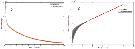
Figure 7. Verification of the Burger Model: (a) Stress relaxation; (b) Creep.
The results of both experimental and numerical tests were analyzed. The experimental test was conducted on the bitumen to determine its rheological measurements (storage and loss moduli). The test procedure, sample preparation, and results of the laboratory experiments are reported in [32].
Laboratory measurements
Two laboratory test data were used to: (i) measure the dynamic modulus and phase angle of the bitumen for determining the Burgers model parameters [32] and (ii) measure the complex modulus and phase angle of the oil sands formation for validation of the 2D DEM model [13]. The rheological behavior of the bitumen was obtained using the dynamic shear rheometer (DSR) under a stress/strain controlled condition. Behzadfar and Hatzikiriakos [32] recently conducted an experiment to measure the dynamic modulus and phase angle of bitumen at different temperatures, applying frequencies from 0.005 to 500 rad/s using the DSR. The temperature range of the experimental testing varied from -30°C to 90°C. The dynamic modulus and phase angle of bitumen is depicted in Figure 8 at selected temperatures (-30, 0, 10, 30, 60 and 90°C).
Figure 8(a) shows that for the same frequency, the magnitude of the dynamic modulus generally decreases with an increase in temperature. Also, at the same temperature, the magnitude of the dynamic modulus increases with an increase in the loading frequency. Conversely, the magnitude of the phase angle increases with an increase in temperature from -30 to 30°C for the same frequency but decreases with a temperature range of 60 to 90°C.
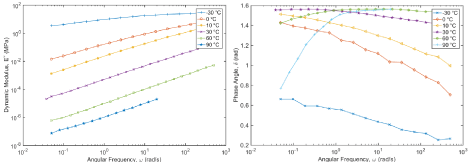
Figure 8. Measured rheological properties of bitumen at selected temperatures: (a) Dynamic modulus versus frequency; (b) Phase angle versus frequency [32].
The nonlinear least squares (lsqnonlin) solver provided in the MATLAB optimization toolbox was utilized for minimizing the objective function given in Equation (17) and subject to Equation (18-19). The microscale model parameters fitted to the bitumen data are listed in Table 1.
Figure 9 shows the quality of fit of the Burger model to bitumen measurements obtained using the DSR at different temperatures. The figure shows that this model yields a good fit to the experimentally obtained dynamic shear modulus at 0 and 30°C. A less perfect fit still within the acceptable limits is obtained at -30°C.
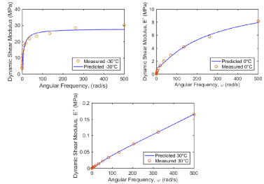
Figure 9. Measured and predicted dynamic shear moduli.
DEM simulation of cyclic uniaxial compressive test for oil sands
A series of uniaxial compressive sinusoidal dynamic loading tests were conducted with the viscoelastic model developed in this study. Table 2 list the viscoelastic model input parameters and other relevant data used for the simulation. The compressive dynamic loading was applied to the top and bottom platens of the digital sample, shown in Figure 3(b), while the two vertical boundary walls were fixed in all directions.
The simulation test involves two stages: (i) an isotropic consolidation, and (ii) uniaxial compressive sinusoidal loading. Before the cyclic uniaxial compression testing, the digital sample was brought to equilibrium under an isotropic stress state. The sample was loaded in a strain-controlled manner were the boundary walls are adjusted using a servo-controlled mechanism to achieve a target confining stress [39]. In this study, haversine stress at different frequencies (10, 7, 5, and 3 Hz) was applied to the loading platens. Both the vertical and horizontal walls moved to gradually apply the required stress. Results for the viscoelastic DE simulation of oil sand material with the corresponding model parameters under compressive dynamic sinusoidal loading are presented in Figures 10 to12.
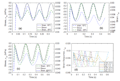
Figure 10. Strain response under constant stress amplitude loading due to application of three loading cycles for each loading frequency and temperature: (a) 10 Hz, (b) 7 Hz, (c) 5 Hz, (d) Strain response at given temperatures and frequencies.
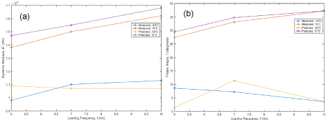
Figure 11. Measured and predicted: (a) Dynamic modulus, (b) Phase angle.
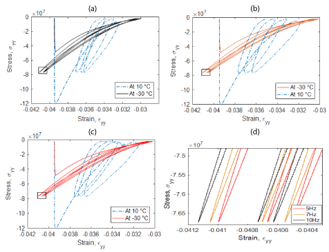
Figure 12. Hysteresis loop at corresponding loading frequencies: (a) 10Hz; (b) 7 Hz; (c) 5 Hz and (d) Inset plot of the corresponding frequencies at -30°C.
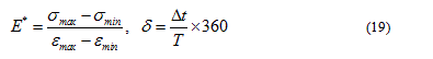
Figure 10 presents the applied sinusoidal compressive loading and the corresponding strain calculated from the displacement of the top and bottom platens. Dynamic modulus  and phase angle
  are calculated from the applied stress and strain response plots in Figure 10 using equation (20):
 are the applied maximum and minimum stress,
  are the maximum and minimum predicted strain response,
  is the time difference between two adjacent peak stress and strain, and T is the loading period, which is the inverse of the loading frequency. The predicted and measured
  and
and  are plotted in Figure 10.
High strain accumulation was observed for the first loading peak point at 10°C rather than at -30°C, but the accumulation decreases gradually as the frequency and loading cycle increases as shown in Figure 10. Generally, for the same loading frequency, the magnitude of the strain decreases as loading frequency and temperature increases. As expected, the oil sand material becomes softer at a higher temperatures, and thus, undergoes high deformation under loading. The viscoelastic response of the oil sand material is depicted in the reduction of strain accumulation with the increase of loading cycle for both temperatures, as shown in Figure 10(d). The reduction in maximum and minimum strain peak as the loading cycle increases is due to the slippage and rearrangement of the discrete quartz particles under loading. This phenomenon leads to some permanent deformation on the removal of the load.
At -30°C, the maximum strain peak decreases from -0.030 to -0.03065 as the loading frequency decreases. Conversely, the minimum strain value increases as the loading frequency increases from -0.04112 to -0.0405. However, at 10°C, the maximum strain decreases from -0.03247 to -0.03505 (a difference of 7.9%) as loading frequency decreases. On the other hand, the minimum strain value ranges from -0.0326 to -0.03772, a decrease of 13.6%. The results indicate that the rate of loading and temperature affects the deformational behavior of the oil sand material. This observation was also reported in field studies conducted by Dehmoobed Sharif-abadi and Grain Joseph [44].
Figure 11 presents the predicted versus experimentally measured [13] dynamic modulus and phase angle for an oil sand material. The model prediction compared well with the measured phase angle at 10°C, while it was higher than the measured dynamic modulus at -30°C. On the other hand, the measured dynamic modulus at -30°C was close to the predicted model.
The stress/strain response behavior (i.e., hysteresis loop) is presented in Figure 11 at the corresponding loading frequencies (5, 7, and 10 Hz).
The area under the loop decreases with increasing loading frequency at -30°C, as shown Figure 12(d). However, the area under the loop increases as loading frequency decreases. This implies that the viscoelastic dissipated energy increases with cyclic loading.
This paper modeled and simulated the linear viscoelastic discrete element behavior for oil sands material based on Burger’s element model. The microstructure was captured by digitizing a two-dimensional scanning electron image to delineate the different constituents of the oil sand material. To study the micromechanical behavior within the material, three types of contacts were considered: aggregate-aggregate, aggregate-bitumen, and aggregate-water-bitumen contacts. The quartz aggregates were modeled as a rigid disc and the linear contact model was defined at the interaction among the aggregates. The time- and temperature-dependent bitumen was modeled with viscoelastic material model. Contact interactions within the bitumen and bitumen-quartz was defined with the Burger’s model. A nonlinear optimization technique based on minimizing the sum of squares of errors was developed to calibrate the microscale model parameters from lab-based macroscale material properties. A dynamic sinusoidal loading with constant amplitude was applied to the bottom and top platen to simulate the viscoelastic material behavior of the oil sands with the calibrated model parameters.
The following can be concluded from the results of this study:
- The aggregate shape and PSD responsible for permanent deformation were accounted for in this micromechanical model. Thus, it can simulate the discrete mechanical behavior of oil sand material;
- Oil sand material can be simulated with a viscoelastic model based on Burger’s contact model over cyclic loading. It accounts for the loading rate and temperature dependency of the material;
- The micromechanical and microstructural viscoelastic model developed in this study can predict the dynamic modulus and phase angle of the material with a maximum error of 13.6%;
In the future, the following work will be addressed in ongoing studies: (i) construct a master curve to be used to model the temperature effects of oil sands material and (ii) quantitatively determine the capillary force at the aggregate-water-bitumen interface and decide if it should be included in the model.
The authors would like to acknowledge the financial (PFC software loan) and technical support by the Itasca Consulting Group Inc., Minnesota through the Itasca Education Partnership program (IEP). The first author would like to thank Mr. Sacha Emam of the Itasca International Inc for his valuable technical support and insight into PFCs model development and implementation.
- Takamura K (1982) Microscopic structure of Athabasca oil sand. Can J Chem Eng 60: 538-545.
- Czarnecki J, Radoev B, Schramm LL, Slavchev R (2005) On the nature of Athabasca Oil Sands. Adv Colloid Interface Sci 114-115: 53-60. [Crossref]
- Dusseault MB, Morgenstern NR (1978) Morgenstern. Shear strength of Athabasca Oil Sands. Canadian Geotechnical Journal 15: 216-238.
- Bowman C (1967) Discussion to the Tar Sands Section in 7th World Petroleum Congress, Mexico City, pp:561-650.
- Harris MC, Sobkowicz JC (1977) Engineering Behaviour of Oil Sand. The oil sands of Canada-Venezuela pp:270-281.
- Joseph T, Hansen G (2002) Oil sands reaction to cable shovel motion. CIM bulletin 95: 62-64.
- Frimpong S, Thiruvengadam M (2016) Multibody Dynamic Stress Simulation of Rigid-Flexible Shovel Crawler Shoes. Minerals 6: 61.
- Wan RG, Chan DH, Kosar KM (1991) A Constitutive Model for The Effective Stress-Strain Behaviour of Oil Sands.
- Samieh AM, Wong RCK (1997) Deformation of Athabasca oil sand at low effective stresses under varying boundary conditions. Canadian Geotechnical Journal 34: 985-990.
- Li P, Chalaturnyk RJ (2005) Geomechanical Model of Oil Sands presented at the International Thermal Operations and Heavy Oil Symposium, Calgary, Alberta, Canada.
- Anochie-Boateng J, Tutumluer E, Carpenter S (2008) Permanent Deformation Behavior of Naturally Occurring Bituminous Sands. Transportation Research Record: Journal of the Transportation Research Board 2059: 31-40.
- Anochie-Boateng J, Tutumluer E (2014) Advanced Testing and Characterization of Shear Modulus and Deformation Characteristics of Oil Sand Materials. J Test Eval 42: 1-12.
- Anochie-Boateng J, Tutumluer E, Carpenter SH (2010) Case study: Dynamic modulus characterization of naturally occurring bituminous sands for sustainable pavement applications. International Journal of Pavement Research and Technology 3: 286-294.
- Cundall PA (1971) A computer model for simulating progressive, large scale movements in blocky rock systems Proceedings of the international symposium on rock fractures," Nancy, France II-8, pp: 1-12.
- Chang KNG, Meegoda JN (1997) Micromechanical Simulation of Hot Mix Asphalt. Journal of Engineering Mechanics 123: 495-503.
- Horner DA (1997) Application of DEM to micro-mechanical theory for large deformations of granular media " PhD Dissertation, Civil Engineering, University of Michigan, Ann Arbor, Michigan.
- Gbadam E, Frimpong S (2014) Bench Structural Integrity Modeling of Oil Sands for Optimum Cable Shovel Performance. J Powder Metall Min 3: 2.
- Brown O, Frimpong S (2012) Nonlinear finite element analysis of blade-formation interactions in excavation. Mining Engineering.
- Yong R, Fattah E (1976) Prediction of wheel-soil interaction and performance using the finite element method. Journal of Terramechanics 13: 227-240.
- Perumpral JV, Liljedahl J, Perloff W (1971) The finite element method for predicting stress distribution and soil deformation under a tractive device. Transactions of the ASAE 14: 1184-1188.
- Liu C, Wong J (1996) Numerical simulations of tire-soil interaction based on critical state soil mechanics. Journal of Terramechanics 33: 209-221.
- Abbas A, Masad E, Papagiannakis T, Harman T (2007) Micromechanical Modeling of the Viscoelastic Behavior of Asphalt Mixtures Using the Discrete-Element Method. Int J Geomech 7: 131-139.
- Sousa J, Weissman SL, Sackman JL, Monismith CL (1993) Nonlinear elastic viscous with damage model to predict permanent deformation of asphalt concrete mixes.
- Rothenburg L, Bathurst RJ (1991) Numerical simulation of idealized granular assemblies with plane elliptical particles. Computers and Geotechnics 11: 315-329.
- Liu Y, Dai Q, You Z (2009) Viscoelastic model for discrete element simulation of asphalt mixtures. Journal of Engineering Mechanics 135: 324-33.
- Abbas A, Masad E, Papagiannakis T, Shenoy A (2005) Modelling asphalt mastic stiffness using discrete element analysis and micromechanics-based models. International Journal of Pavement Engineering 6: 137-146.
- Buttlar W, You Z (2001) Discrete element modeling of asphalt concrete: microfabric approach. Transportation Research Record: Journal of the Transportation Research Board 1: 111-118.
- Dai Q, You Z (2007) Prediction of creep stiffness of asphalt mixture with micromechanical finite-element and discrete-element models. Journal of Engineering Mechanics 133: 163-173.
- Cai W, McDowell GR, Airey GD (2014) Discrete element visco-elastic modelling of a realistic graded asphalt mixture. Soils and Foundations 54: 12-22.
- Kim H, Wagoner MP, Buttlar WG (2008) Simulation of fracture behavior in asphalt concrete using a heterogeneous cohesive zone discrete element model. Journal of Materials in Civil Engineering 20: 552-63.
- Tannant DD, Wang C (2002) Numerical and experimental study of wedge penetration into oil sands. CIM bulletin 95: 65-68.
- Behzadfar E, Hatzikiriakos SG (2013) Viscoelastic properties and constitutive modelling of bitumen. Fuel 108: 391-399.
- Cundall PA, Strack OD (1979) A discrete numerical model for granular assemblies. Geotechnique 29: 47-65.
- Zhu HP, Zhou ZY, Yang RY, Yu AB (2007) Discrete particle simulation of particulate systems: theoretical developments. Chemical Engineering Science 62: 3378-3396.
- Obermayr M, Dressler K, Vrettos C, Eberhard P (2013) A bonded-particle model for cemented sand. Computers and Geotechnics 49: 299-313.
- Oetomo JJ, Vincens E, Dedecker F, Morel JC (2016) Modeling the 2D behavior of dry-stone retaining walls by a fully discrete element method. Int J Numer Anal Methods Geomech 40: 1099-1120.
- Cundall PA (1974) A computer model for rock-mass behavior using interactive graphics for the input and output of geometrical data. Minnesota Univ Minneapolis Dept of Civil and Mining Engineering.
- Crain ER (1978) Crain's Petrophysical Handbook.
- Itasca Consulting Group Inc (2014) PFC-Particle Flow Code, Ver. 5.0," ed. Minneapolis: Itasca.
- Yu H, Shen S (2013) A micromechanical based three-dimensional DEM approach to characterize the complex modulus of asphalt mixtures. Constr Build Mater 38: 1089-1096.
- Papagiannakis A, Abbas A, Masad E (2002) Micromechanical analysis of viscoelastic properties of asphalt concretes. Transportation Research Record: Journal of the Transportation Research Board 1: 113-120.
- Baumgaertel M, Winter HH (1989) Determination of discrete relaxation and retardation time spectra from dynamic mechanical data. Rheologica Acta 28: 511-519.
- Abbas AR (2004) Simulation of the micromechanical behavior of asphalt mixtures using the discrete element method. Washington State University.
- Sharif-abadi AD, Joseph TG (2010) An oil sand pseudo-elastic model for determining ground deformation under large mobile mining equipment. Geotechnical and Geological Engineering 28: 471-481.