Take a look at the Recent articles

Abstract

The aim of this studywas to evaluate the blood vascular network of the retina and its regions in diabetic patients with and without signs of mild early diabetic retinopathy by using number of bifurcation points, fractal and multifractal methods. We used 33 segmented images of retinographies, 28 corresponding to the retinographies that did not show any sign of diabetic retinopathy and 5 diagnosed with non-proliferative diabetic retinopathy(NPDR). The segmented images were obtained from the DRIVE (Digital Retinal Images for Vessel Extraction) database. The segmented images of retinal blood vessels were skeletonized and fractionated into nine equal regions. Later, the skeletonized images were assessed by using the following methods: number of bifurcation points, box-counting dimension, information dimension, lacunarity parameter and multifractal analysis. The retinas and their regions of control group (diabetic without NPDR) were statistically compared to those of the NPDR by using the Z-test and the Mann-Whitney test.The multifractal analysis showed that skeletonized images of retinal vessels and its nine regions follow a multifractal behavior. In our hands, neither the fractal method nor the number of bifurcation points disclosed statistically significant differences (p>0.05). Noany difference was observedin the retinal vascular network between diabetic patients with or without NPDR.

Key words

 non-proliferative diabetic retinopathy, vascular network, fractal analysis,multifractal analysis, lacunarity

Introduction

Among the ophthalmopathies, the diabetic retinopathy is one of the causes of vision impairment and blindness[1]. This secondary microvascular complication of diabetes mellitus occurs due to the hyperglycemia that promotes structural and functional alteration of retinal capillaries [2]. The early stage of retinopathy is termed as non-proliferative diabetic retinopathy, a disease characterized by microaneurysms, hemorrhages and capillary closure [2,3]. The proliferative phase is characterized by neovascularization, increasing of ischemic regions, hemorrhage in the vitreous cavity andtractional retinal detachment [2,4].

The retinal vascular network owns a fractal structure, the vascular branching process presents self-similarity and scaling. A fractal object or process is characterized by the following properties: self-similarity, scaling, fractal dimension [5,6].Several works have used the fractal geometry to study the retinal vascular network [7,8]. Doubalet al.[9] have obrtained the fractal dimension of retinal vessels in the lacunar stroke and Cavallariet al.[10]in the cerebral autosomal dominant arteriopathy with subcortical infarcts and leukoencephalopathy (CADASIL). Avakianet al.[11],Kunickiet al.[12] and Ţăluet al. [13] have used fractal methods to identify non-proliferative diabetic retinopathy (NPDR), however obtaining contradictory results.

Since the fractal dimension describes how much space is filled, but does not indicate how the space is filled by the fractal structure, the lacunarity can solve this problemby making a distinction between different objects with the same fractal dimension [14,15]. The lacunarity is a parameter that indicates the distribution of gap sizes throughout the object embedded in an image, it is able to identify different fractal structures that have the same fractal dimension [14]. This parameter has been used as a tool in the characterization of retinal vascular network. Landiniet al.[16] have employed the lacunarityto identify the occlusion of the artery and retinal vein, whereas Tăluet al.[17]have used it to diagnose amblyopic eyes.

Some studies have currently characterized some objects as multifractal structures (objects that have different fractal dimensions) instead of monofractal, as regarded in the previously mentioned studies. An object is consideredmultifractal when its different regions have different fractal properties [18]. Researchers have demonstrated the network of vessels ofthe retina as a multifractal object, a fact which has been proved through generalized dimensions and singularity spectrum [15,19]. Furthermore,the singularity spectrum has the capacity to evidence the disorders in the retinal vascular architecture with diseases [19].

The aim of this studywas to assess the network of blood vessels of the retina and its regions with and without signs of mild early diabetic retinopathy by using the number of bifurcation points and fractal methods,such as box-counting dimension, information dimension,lacunarity parameter (complementary tool of fractal methods)and multifractal analysis: generalized dimensions and singularity spectrum.

Material and methods

Retinal images

The images were obtained from the DRIVE (Digital Retinal Images for Vessel Extraction) [20] database (http://www.isi.uu.nl/Research/Databases/DRIVE/).We used 28 retinographies(control group) which do not show any sign of diabetic retinopathy(Figure 1A) and 5 diagnosed with mild early diabetic retinopathy, non-proliferative diabetic retinopathy (NPDR) (Figure1B).The images were acquired from diabetic patients between 25-90 years of age, by using a Canon CR5 non-mydriatic 3CCD camera with a 45 degree field of view (FOV). Each image was captured by using 8 bits per color plane at 768 by 584 pixels. The FOV of each image is circular with a diameter of approximately 540 pixels and each image has been JPEG compressed.

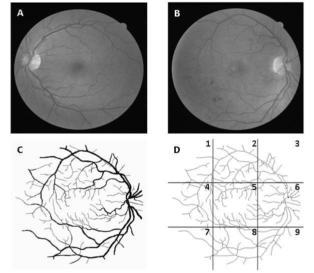
Figure 1. Image of normal retina (A), image with signs of mild early diabetic retinopathy (B), segmented image B (C) and same skeletonized image divided into 9 regions: 1 - superotemporal, 2 - superior, 3 - nasal superior, 4 - temporal, 5 - macular, 6 - optic disc, 7 - inferotemporal,  8 – inferior and 9 – nasal inferior (D).

Skeletonization and separation by region

The manually segmented images of retinal vessels (Figure 1C) were also obtained from DRIVE. The segmented images of vessels (565x586 pixels) were skeletonized bythe software Matlab® version 7.8 (MathWorks, Natick, Ma, U.S.A). Each image was fractionated into nine equal regions (Figure 1D) by the software Adobe Image Ready 7.0.1. Figure 1shows the retina in gray scale, segmented, skeletonized and divided by region (nasal superior, optic disc, nasal inferior, superior, macular, inferior, superotemporal, temporal and inferotemporal).  

Counting of bifurcation points

The bifurcation point is where a blood vessel originates other vessels. The number of bifurcation points is a method that informs about the amount of branching, showing the vascular multiplication. The procedure proposed here is an optional method to measure the blood vascularization degree as another morphometric parameter to evaluate the vascular architecture (density, length, diameter of vessels). The bifurcation points were determined from skeletonized images of the retinas and their respective regions for both groups. The identification process was confirmed in the original retinographies to reduce the possibility of quantifying artifacts or overlapping of vessels.  

Fractal dimension methods

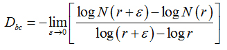
Two methods were used to calculate the fractal dimension of retinal blood vessels, the box-counting dimension (D_bc) and the information dimension (D_inf) bythe software Benoit 1.3 Fractal Analysis System (Trusoft, St. Petersburg, FL, USA).For the box-counting dimension (D_bc), the skeletonized image was covered with a number of boxes (N (r)) containing at least one pixel of the image. The procedure was repeated with boxes of different sizes and plotted in a double log graph of N (r) inrelation to the sides of boxes r [21]. The slope of this relationship with inverted signal is the box-counting dimension:

                               (1)         

in whichεisaninfinitesimal variation in the box sizes. The calculations ofD_bc used 19 sets of different size boxes, the length of the largest box side being 270 pixels and the reduction coefficient of the box size 1.3.

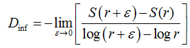
In the information dimension (D_inf), skeletonized images were also covered by boxes, but taking into account the relative probability of occupancy of the elementary boxes used to cover the fractal object:

                                             (2)

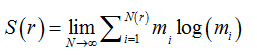
where

                                                  (3)

is called the Kolmogorov entropy. N is the number of boxes, m_i= M_i / M, and M_i is the number of pixels in the n^th box, M is the total number of pixels on the fractal object, r is the side of boxes andε is a infinitesimal variation in boxsizes [21].The calculations ofD_inf used 8 sets of different size boxes, the length of the largest box side being 270 pixels and the reduction coefficient of box size 2.0.

Figure 2 shows the box-counting dimension graph (Figure 2A) and information dimension (Figure 2B).

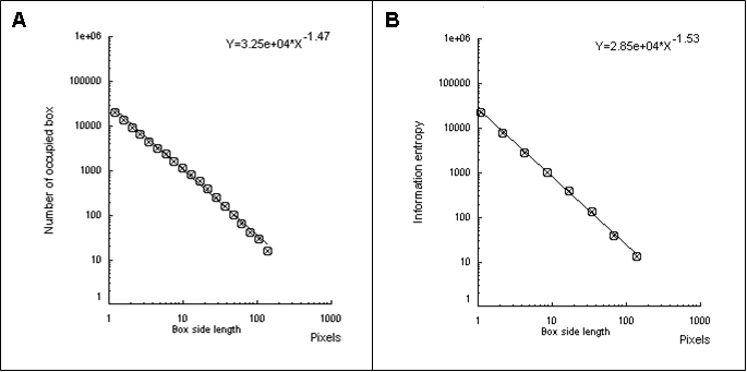
Figure 2. The box-counting dimension is the slope with inverted signal obtained by the number of occupied boxes according to the size of the sides of the boxes (A). The information dimension is the slope with inverted signal obtained by information entropy (Kolmogorov entropy) according to the size of the sides of the boxes (B).

Lacunarity parameter

To evaluate the lacunarity parameter of the images of the retinal vessels, we used the software Image J (Wayne Rasband, National Institutes of Health in Bethesda, Maryland, USA)withthe FracLacplug-in (A. Karperien – Charles Sturt University, Australia). Lacunaritywas obtained by measuring thegap dispersion inside an image; in other words, it was related to the pixel distribution of an object in an image. The quantification was achieved as in the box-counting method. In this case, however,different directions to the set of boxes (g) was also used.

The mean value to the lacunaritywas calculated as follows:

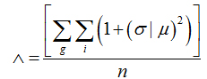
                                                        (4)

whereσ is the standard deviation and μ is the mean of pixels per box with size r, in a box-counting at adirection g,n being the number of box sizes. The sum is done over all values of r and g.

Multifractal analysis

Software Image J withFracLacplug-in was also used to calculate the multifractality of retinalvasclarization. The multifractal structure is characterized by obtaining the generalized dimension D_q, which is related to a value of q. Variable q is the exponent that expresses the fractal properties in different scales to an object, ranging between -∞ and + ∞. The plot ofD_q versus q is generally sigmoidal and decreasing to a multifractal structure. Some studies consider determined values D_qthat isD₀, D₁ and D₂, which depict the multifractality of an object when condition D₀ ≥ D₁ ≥ D₂is satisfied. Values D_qdepict the multifractal object that can be compared by the single fractal dimension method, soD₀ can be considered as capacity dimension, D₁can be related to the information dimension and D₂to the correlation dimension[19].In our study, values were generated fromD_-10 to D₊₁₀, in other words, qvalues ranged between -10 and +10, where all dimensions were statistically tested.D_qwas calculated as follows:

                                                         (5)         

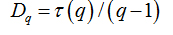
can be defined as:            

                                 (6)

where 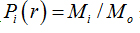is density, M_iis the number of pixels within the i^th box and M₀ is the number of pixels for all image. is the density for all boxes (i) at a determined scaler.

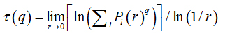
Another way to calculate the multifractal spectra is through the relationship between parameters f(α)versus α, where

                                                                  (7)

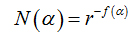
N(α) is the number of boxesfor which probability P_i(r) of finding a pixel within a given region i scales as

                                                                                                                                                (8)

f(α)is the fractal dimension to the all regions with singularity strengths between α and α + dα, where α takes on values between -∞ and + ∞.

These variables were obtained by Legendre transformation from τ into q, as described below:

                                         (9)

and        

                                                                                        (10)

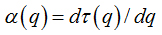
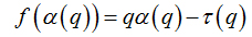
Also, α (q) and f (α(q)) can be calculated by usingthe following equations:

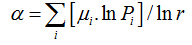
                                   (11)

and

                                       (12)

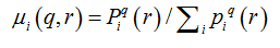
where

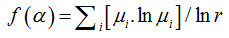
                                  (13)

P_i^q(r) is the probability of pixels inthe i^th box for the exponent q. For a multifractal object, plot α versus f(α) fits a parabola with concavity turned down.

From values α,it was possible to calculatethe extension of singularity length Δα and the curve asymmetry of singularity spectrum.Extension of singularity length Δαis defined as follows:

                                             (14)

α_max (highest value ofα) andα_min (lowestvalue ofα) indicate the fluctuation of minimum and maximum probability of pixels, respectively. The higher the Δα, the larger the probability distribution; furthermore, the multifractality is stronger and the pixel distribution of image is morecomplex [22,23].

                The curve asymmetry of singularity spectrum (A)was calculated according to the following expression:

                                   (15)

The curve of singularity spectrumis symmetric to A=1, the curve is left-skewedif A>1 and is right-skewed if A<1. When the spectrum is left-skewed, it means that there is stronger presence of high fractal exponents and significant fluctuation; otherwise, it indicates the domain of low exponents and slightfluctuation [23].

Statistic analysis

The Shapiro-Wilk’s test was used to calculatethe number of bifurcations, fractal dimensions, lacunarity parameters, generalized dimensions,Δα and parameter A (curve asymmetry of the singularity spectrum). The Shapiro-Wilk’s test was used to choose between a parametric test or nonparametric, in order to make a comparison between the different regions and the whole retina with and without NPDR within the two groups. The Z-test was used when the group had a normal distribution and the Mann-Whitney test for a non-normal distribution. The Z-test, here, is a method to inform if the distribution of group with NPDR had the same behavior of the distribution of group without NPDR, this test is acceptable to conditions in that one of the groups possesses a low number of samples while the other has the highest number of samples. 

Results

Number of bifurcation points

Table 1 shows the number of bifurcation points, in whichp is the value of the significance level to the Z-test or the Mann-Whitney test (with asterisks). For regions such as optic disc, nasal inferior and temporal in which the controlgroup did notpresent a normal distribution, the Mann-Whitney test (nonparametric test) was used. For other regions and the whole retina in which the controlgroup presented normal distribution, the Z-test was used. The statistical tests did not show any difference in the bifurcation points between the control group and the NPDR group (p>0.05).

Retinal region	Control	NPDR	p-value
Whole	103.4 ± 22.6	91.4 ± 13.0	0.297
Nasal superior	5.89 ± 1.83	7.40 ± 2.70	0.794
Optic disc	17.60 ± 4.48	17.6 ± 5.41	0.723*
Nasal inferior	5.53 ± 1.91	4.80 ± 2.16	0.540*
Superior	15.6 ± 5.51	15.0 ± 3.16	0.456
Macular	17.8 ± 6.53	14.4 ± 3.50	0.296
Inferior	13.9 ± 3.59	12.6 ± 2.30	0.356
Superotemporal	6.67 ± 2.73	5.80 ± 0.44	0.374
Temporal	14.2 ± 5.03	10.4 ± 4.77	0.158*
Inferotemporal	6.03 ± 2.60	3.40 ± 2.07	0.155

Table 1. Number of bifurcation points of all regions and whole retina of control group and NPDR
P-values with asterisks indicate where the Mann-Whitney test was used; Z-normal test was used in the other regions. The Shapiro-Wilk’s test was used to test the normality.

Box-counting dimension and information 

The first step to make the statistical analysis of fractal dimensions of the two groups was to test whether the segmentations represented the original images of the retinasaccurately. We selected ten segmented images of the DRIVE made by one observer, carried outtheskeletonization for the control group and compared it to the skeletonization of the same ten images segmented manually by another observer. Figure 3 represents the box-counting dimensions (3A) and information (3B) to segmented and skeletonized images, respectively;t-student test showed that for both observers there were no significant differenceneither between the segmented images (p=0.82for box-counting dimension and p=1.0for information dimension) northe skeletonized ones (p=1.0for box-counting dimension and p=0.68for information dimension). These results showed that the manual segmentation is a reliable method and can be considered as gold standard. Table 2 shows the fractal dimensions (box-counting dimension and information) of the control group and NPDR.  In this case, neither the whole retina nor its different regions in the control group displayed difference to the NPDR group (p>0.05).

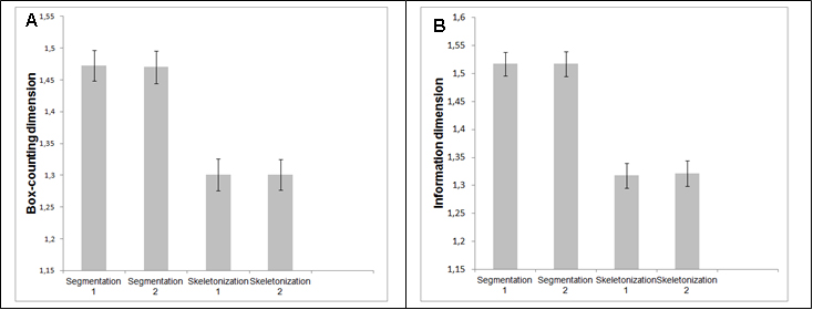
Figure 3. Box-counting dimension (A) and information dimension (B) of the network of retinal vessels by 2 different observers.

Retinal region	Dbc of control group	Dbc of NPDR group	p- value of Dbc	Dinf of control group	Dinf of NPDR group	p-value of Dinf
Whole	1.29 ± 0.02	1.28 ± 0.02	0.30	1.31 ± 0.02	1.30 ± 0.02	0.39
Nasal superior	1.07 ± 0.03	1.08 ± 0.02	0.67	1.10 ± 0.04	1.13 ± 0.02	0.71
Optic disc	1.14 ± 0.02	1.14 ± 0.04	0.49	1.21 ± 0.03	1.21 ± 0.04	0.49
Nasal inferior	1.03 ± 0.03	1.02 ± 0.03	0.38	1.07 ± 0.04	1.05 ± 0.03	0.28
Superior	1.09 ± 0.03	1.07 ± 0.01	0.33	1.14 ± 0.04	1.12 ± 0.02	0.31
Macular	1.10 ± 0.04	1.10 ± 0.02	0.43	1.15 ± 0.03	1.15 ± 0.02	0.45
Inferior	1.08 ± 0.02	1.06 ± 0.03	0.23	1.13 ± 0.03	1.11 ± 0.02	0.23
Superotemporal	1.01 ± 0.04	1.02 ± 0.03	0.50	1.06 ± 0.05	1.06 ±  0.02	0.51
Temporal	1.06 ± 0.04	1.04 ± 0.06	0.30	1.11 ± 0.04	1.08 ± 0.07	0.22
Inferotemporal	1.03 ± 0.03	1.00 ± 0.05	0.23	1.07 ± 0.03	1.05 ± 0.07	0.22

Table 2. Fractal dimensions of all regions and whole retina of the control group and NPDR
All regions were submitted to the Z-normal test. The Shapiro-Wilk’s test was used to test the normality.

Lacunarity parameter

Table 3 depicts the lacunarity values. Some regions of the two groups were submitted to the Mann-Whitney test (values with asterisks) and others to the Z-test. Statistically, there was no difference between the lacunarity parameters for the control group and NPDR (p>0.05).The Shapiro-Wilk’s test was used to test the normality.

Retinal region	Control group	NPDR group	p-value
Whole	0.219 ± 0.016	0.211 ± 0.008	0.33
Nasal superior	0.331 ± 0.064	0.309 ± 0.058	0.37
Optic disc	0.246 ± 0.030	0.267 ± 0.044	0.75
Nasal inferior*	0.344 ± 0.072	0.326 ± 0.080	0.54
Superior*	0.227 ± 0.047	0.208 ± 0.022	0.58
Macular	0.216 ± 0.027	0.249 ± 0.020	0.88
Inferior	0.237 ± 0.030	0.230 ± 0.023	0.41
Superotemporal	0.300 ± 0.049	0.321 ± 0.066	0.66
Temporal	0.234 ± 0.024	0.242 ± 0.018	0.62
Inferotemporal*	0.291 ± 0.037	0.361 ± 0.131	0.27

Table 3. Lacunarity parameters of all regions and whole retina of the control group and NPDR
The Mann-Whitney test was used in the regions with asterisks and the Z-normal test was used in the others. The Shapiro-Wilk’s test was used to test the normality.

Multifractal analysis

There wasa statistical difference in dimension D_-1 in the inferotemporal region (p=0.04 to the Z-test), whilst other generalized dimensions of the same region corresponding to both groups were not significantly different. The generalized dimensions of other regions and the whole retina did not show any statistically significant difference. Table 4 presents the mean and standard deviations of following generalized dimensions for bothgroups: D_-10, D₀, D₁, D₂ and D₁₀.

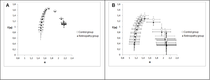
Figure 4 shows two graphs that represent the mean and standard deviations of generalized dimensions (D_q) versus variable qfor the whole retina and for the inferotemporal region in which there was a statistical difference indimension D_-1.The plots followed a sigmoid fit, outlining a multifractality for blood vascular network of the retina and its regions. Each graph has two plots, one that depicts the control group and the other showing the retinopathy group. Figure 4A representsD_q versus q for the whole retina inthe two groups (control and NPDR), showing a behavior with less oscillation (low standard deviation) compared to Figure 4B (inferotemporal region). Figures 5A and 5B represent the graph of f(α) versus α to the whole retina and the inferotemporal region respectively, in which each graph presents the group with and without NPDR. The graphs showed the typical behavior of multifractal structures, aparabole with concavity facing down.

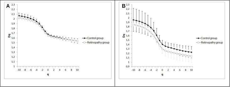
Figure 4. Generalized dimensions of the control group and NPDR. 4A represents the whole retina and 4B represents the inferotemporal region.

Mean values with standard deviations of Δα and A are shown in Table 5. Values ​​of parameter Δα represent the mulifractality of the blood vascular network of the retina and its regions. Tests revealed no statistically significant differences for parameter Δα between the control group and the one with NPDR. In relation to the mean values with the respective standard deviations of parameter A​​, the retinas and all their regions for the two groups were observed to have values ​​of A <1, or, in other  words, the curve of singularity spectrum f (α) versus α was right-skewed. Thus, there was a greater presence of low fractal exponents and low fluctuations. For parameter A, the statistical tests revealed no significant difference between the control group and the one with NPDR.

Table 4. D_-10, D₀, D₁, D₂ e D₁₀ of all regions and whole retina of the control group and NPDR.
Values p with asterisks indicate the regions compared by using the Mann-Whitney test, whereas the Z-normal test was used for other regions

2021 Copyright OAT. All rights reserv

Retinal region	Δα			A
	Control group	Group NPDR	P	Control group	Group NPDR	p
Whole	0.699±0.09	0.645±0.08	0.27	0.548±0.15	0.498±0.066	0.68*
Nasal superior	1.121±0.46	1.378±0.56	0.33*	0.585±0.44	0.444±0.085	0.67*
Optic disc	0.725±0.13	0.815±0.18	0.75	0.476±0.20	0.552±0.266	0.70*
Nasal inferior	0.844±0.23	1.154±0.63	0.9	0.623±0.33	0.492±0.201	0.34
Superior	0.698±0.15	0.725±0.12	0.57	0.450±0.16	0.370±0.093	0.33*
Macular	0.879±0.12	0.846±0.2	0.39	0.677±0.17	0.611±0.143	0.33*
Inferior	0.783±0.18	0.771±0.14	0.47	0.578±0.21	0.672±0.181	0.67
Superotemporal	1.458±0.64	1.650±0.64	0.62	0.463±0.17	0.457±0.199	0.48
Temporal	0.807±0.19	0.886±0.12	0.66	0.516±0.14	0.419±0.124	0.25
Inferotemporal	0.951±0.36	0.940±0.16	0.64*	0.495±0.15	0.458±0.073	0.40

Table 5. Values Δα ​​and asymmetry values ​​of singularity spectrum (A) of all regions and whole retina of the control group and the one with NPDR
Values p ​​with asterisks indicate the regions compared by using the Mann-Whitney test. For the other regions. the Z-normal test was used.

Discussion 

The non-proliferative diabetic retinopathy is characterized by microaneurysms, hemorrhages and capillary closure [2,3]. The rise in hemodynamic alterations and compensatory mechanisms due to the presence of such signs may promote changes in vascular architecture. In this paper, we have used methods that are capable of identifying the geometric complexity of the blood vascular network.

The fractal dimension is a statistical descriptor of the space-filling pattern and density serving as a tool capable of evaluating the vascular development and thereforeit canhelp in the diagnosis of diseases related to the vascular disorders [7,24,25]. The retinal vascular network has a fractal dimension that ranges between 1 and 2, as being close to 2 indicates a more complex networkor higher vascular density. For instance, Doubalet al.[9] have associated a low value of fractal dimension of retinal vessels to the lacunar stroke subtype. Also, according to Cavallariet al. [10], the decrease in fractal dimension is related to the reduction incomplexity of retinal vessels, which reflects in the alteration in brain microvessels in patients with CADASIL.

To identify possible vascular alterations not disclosed by fractal dimensions, the parameter of lacunarity,which has the capacity to recognize different fractal structures with the same fractal dimension, was employed, describing how the pixels are organized in the full image. This is a way to measure heterogeneity, as well as the degree of invariance to change of the fractal object in an image. Whereas the fractal dimension indicates how much space is filled by vessels, this parameter (reflected in the distribution of gaps) represents how the vessels fill the space whereinthey are embedded [15]. This parameter has been used to discover alterations in the arteries and retinal veins [16], as well as to diagnose retinas with amblyopia[17]. The lacunarity parameters obtained were not statistically different as regards the normal state and thedisease, thus ratifying the results obtained by using the number of bifurcation points, box-counting and information dimensions.

In the multifractal analysis, only one related value D_-1of the inferotemporal region showed statistical difference between the two groups. We can say that the single exponent q=-1 is not enough to characterize the retinal vascular architecture with NPDR. All generalized dimensions to retinas and their other regions showed no any differences. The multifractal analysis ensures more information about the behavior of the network of blood vessels once it reveals several values that estimate simultaneously the level of geometric complexity or filling of space by the vessels. The graphs infigure 4 present a behavior that defines them as a multifractal structure, represented by the descending sigmoid curve of D_q spectrum (generalized dimensions) versus q for the two groups. In case the object presents constant values for fractal dimensions,graphD_q versus q should be a straight parallel to q axis, and the object must be considered a monofractal structure.

Singularity spectrum f (α) calculates the fractal dimension of the subset of pixels in an image described by a particular exponent, referring to the relative dominance of various fractal exponents involved in the structure [26].Figure 5 showed that spectrum f(α) versus α also represents the multifractality of retinal vessels for both groups; in this case, the spectrum is a parabola with concavity facingdown[27].Stŏsić and Stŏsić [19] have shown that the singularity spectrum (graph f(α) versus α)of retinal vascular network follows a multifractal geometry for both normal and pathological states; they have also shown that a group of retinas with different diseases presented lower singularity compared to normal retinas. In our case, we showed a group diagnosed just with NPDR and that there was no distinct singularity spectrum in relation to the diabetic group without the NPDR(Figure 5). In order to assess the multifractality of the vascular networks of retinas and their regions, length Δα [22,23,26] was used, which was not statistically different when comparing the two groups as observed in Table 5. Another wayto analysethe singularity spectrumis through itscurve asymmetry[23]. As already mentioned, this parameter was not statistically different within the two groups. Moreover,both groups showed values of low fractal exponents (A <1).

The condition D_cap≥ D_inf ≥ D_co has been established for each method that these exponents represent in measuring the fractal processes [28]. In terms of generalized dimensions, this condition can be described as follows:D₀≥ D₁≥ D₂[15,19,29]. Each retina in both groups presented this condition, but when the regions were analyzed, some images from those regions lost this criterion, even fordecreasingD_qvalues with the increase in exponent q.The superiorregion was the one with the highest number of images (7) not following such criterion. All images of the inferior region, macular and nasal superior are within this condition. Nevertheless, we can state that the vascular network of retinal regions presents multifractality,not only the vascular network of the whole retina, but its regions can also be considered a superposition of monofractalstructures [19,30].

The fractal dimensions obtained by the box-counting and information methodsare not ruled by the condition stated by Grassberger and Procaccia [28] in that D_cap ≥ D_inf. Likewise, results obtained byMendonçaet al.[31]; Kunickiet al. [12] and Voinea andPopescu [32] were also found to be out of that condition. Considering that the mass-radius dimension of a structure is higher than the box-counting dimension (capacity dimension) [31,32],Family et al. [7], having obtained a higher correlation dimension than the mass-radius one for retinal blood vascularization, theprinciple D_cap≥ D_inf ≥ D_co was contradicted

Some researches have reported alterations of retinal vascularization in individuals with different states of diabetes,Daxer [33] has utilized the fractal geometry to characterize quantitatively the formation and regression of neovascularization in the diabetic retinopathy. Cheung et al. [34] observed that the increase in the fractal dimension of the retinal vasculature is associated with early NPDR signs in young individuals with type 1 diabetes. Ţăluet al. [13] also found the fractal dimension values slightly lower to the retinal images of normal patients than the values to the patients’ images with NPDR. However, Lim et al. [35] have reported that the fractal dimension of retinal vasculature was not associated with incident early diabetic retinopathy in children and adolescents that possess the type 1 diabetes. In this work, the diabetic patients despite not having the signs that characterize mild early diabetic retinopathy showedvascular network geometry similar to the patients with the retinopathy, according to the results revealed by fractal methods (box-counting dimension, information dimension, generalized dimensions, singularity spectrum and lacunarity parameter) and the number of bifurcation points in skeletonized images of the retinal vascular network. However, contradictory results have been described in other works. Avakianet al. [11]performing fractal analysis in skeletonized images from 60-degree fundus fluorescein angiography, observed that the density values of vessels in normal retina macular region was higher than the vascular density of the retinal macular region with NPDR. Our study corroborates the results obtained by Kunicket al.[12] that showed no difference between retinal images of patients with and without NPDR, utilizing fractal dimension analysis (box-couting and information dimension) in segmented images of the retinal vascular network.Diabetic patients, despite not having the signs that characterize a mild early diabetic retinopathy, show a vascular geometry similar to the patients with the disease, according to the results revealed by fractal methods (box-counting dimension, information dimension, generalized dimensions, singularity spectrum and lacunarity parameter) and the number of bifurcation points. We can suggest the existence ofvascular network alterations before to arise the NPDR, since the retinal fractal dimension in normal individuals is different than in diabeticpatients [36].

Conclusion

According to our fractal analysis (box-counting dimension, information dimension, generalized dimensions, singularity spectrum andlacunarityparameter), as well as the measure of number of bifurcation points did not disclose geometrical alterations inthe retinal vascular network for eithergroup of diabetic patients, with or without non-proliferative diabetic retinopathy.In addition, we have observed thatnotonly the vascular network of wholeretina, butalso its several regionsfollow a multifractal behavior.

Funding sources

We thank the Coordination for the Improvement of Higher Education Personnel - (CAPES) and Foundation of support for Science and Technology of Pernambuco (FACEPE). Edbhergue Ventura Lola Costa was a fellowof CAPES.

References

1. Antonetti DA, Barber AJ, Bronson SK, Freeman WM, Gardner TW, et al. (2006) Diabetic retinopathy seeing beyond glucose-induced microvascular disease. Diabetes 55: 2401-2411. [Crossref]
2. Crawford TN, Alfaro DV 3rd, Kerrison JB, Jablon EP (2009) Diabetic retinopathy and angiogenesis. Curr Diabetes Rev 5: 8-13. [Crossref]
3. Shah CP, Chen C (2011) Review of therapeutic advances in diabetic retinopathy. Ther Adv Endocrinol Metab 2: 39-53. [Crossref]
4. Tremolada G, Del Turco C, Lattanzio R, Maestroni S, Maestroni A, et al. (2012) The role of angiogenesis in the development of proliferative diabetic retinopathy: impact of intravitreal anti-VEGF treatment. Exp Diabetes Res 2012: 728325. [Crossref]
5. Mandelbrot B (1991) Objetos Fractais. Lisboa: Gradiva.
6. Bassingthwaighte JB, Liebovitch LS, West BJ (1994) Fractal Physiology. New York: Oxford University Press.
7. Family F, Masters BR, Platt DE (1989) Fractal pattern formation in human retinal vessels. Physica D 38: 98-103.
8. Azemin MZ, Kumar DK, Wong TY, Kawasaki R, Mitchell P, et al. (2011) Robust methodology for fractal analysis of the retinal vasculature. IEEE Trans Med Imaging 30: 243-250. [Crossref]
9. Doubal FN, MacGillivray TJ, Patton N, Dhillon B, Dennis MS, et al. (2010) Fractal analysis of retinal vessels suggests that a distinct vasculopathy causes lacunar stroke. Neurology 74: 1102 – 1107. [Crossref]
10. Cavallari M, Falco T, Frontali M, Romano S, Bagnato F, et al. (2011) Fractal analysis reveals reduced complexity of retinal vessels in CADASIL. PLoS One 6: e19150. [Crossref]
11. Avakian A, Kalina RE, Sage EH, Rambhia AH, Elliott KE, et al. (2002) Fractal analysis of region-based vascular change in the normal and non-proliferative diabetic retina. Curr Eye Res 24: 274–280. [Crossref]
12. Kunicki AC, Oliveira AJ, Mendonça MB, Barbosa CT, Nogueira RA (2009) Can the fractal dimension be applied for the early diagnosis of non-proliferative diabetic retinopathy? Braz J Med Biol Res 42: 930-934. [Crossref]
13. Talu S, Calugaru DM, Lupascu CA (2015) Characterisation of human non-proliferative diabetic retinopathy using the fractal analysis. Int J Ophthalmol 8: 770-776. [Crossref]
14. Mandelbrot B (1983) The Fractal Geometry of Nature. New York : Freeman.
15. Gould DJ, Vadakkan TJ, Poché RA, Dickinson ME (2011) Multifractal and lacunarity analysis of microvascular morphology and remodeling. Microcirculation 18: 136-151. [Crossref]
16. Landini G, Murray PI, Misson GP (1995) Local connected fractal dimensions and lacunarity analyses of 60° fluorescein angiograms. Invest Ophthalmol Vis Sci 13: 2749-2755. [Crossref]
17. Talu S, Vladutiu C, Popescu LA, Lupascu CA, Vesa SC, et al. (2012) Fractal and lacunarity analysis of human retinal vessel arborisation in normal and amblyopic eyes. HVM Bioflux 5: 45-51. [Crossref]
18. Stanley HE, Meakin P (1988) Multifractal phenomena in physics and chemistry. Nature 335: 405-409. [Crossref]
19. Stosic T, Stosic BD (2006) Multifractal analysis of human retinal vessels. IEEE Trans Med Imaging 25: 1101-1107. [Crossref]
20. DRIVE: Digital retinal images for vessels extraction. (http://www.isi.uu.nl/Research/database/DRIVE:index.php )
21. Costa EVL, Jimenez GC, Barbosa CTF, Nogueira RA (2013) Fractal analysis of extra-embryonic vascularization in japanese quail embryos exposed to extremely low frequency magnetic fields. Bioelectromagnetics 34: 114-121. [Crossref]
22. Shi K, Liu CQ, Ai NS (2009) Monofractal and multifractal approaches in investigating temporal variation of air pollution indexes. Fractals 4: 513-521.
23. Hu MG, Wang JF, Ge Y (2009) Super-resolution reconstruction of remote sensing images using multifractal analysis. Sensors (Basel) 9: 8669-8683. [Crossref]
24. Parsons-Wingerter P, Elliott KE, Clark JI, Farr AG (2000) Fibroblast growth factor-2 selectively stimulates angiogenesis of small vessels in arterial tree. Arterioscler Thromb Vasc Biol 20: 1250-1256. [Crossref]
25. Mancardi D, Varetto G, Bucci E, Maniero F, Guiot C (2008) Fractal parameters and vascular networks: facts & artifacts. Theor Biol Med Model 5: 12. [Crossref]
26. Telesca L, Lapenna V, Macchiato M (2004) Mono- and multifractal investigation of scaling properties in temporal patterns of seismic sequences. Chaos, Solitons and Fractals 19: 1-15.
27. Barabási AL, Vicsek T (1990) Self-similarity of the loop structure of diffusion-limited aggregates. J Phys A: Math Gen 23: L729 - L733.
28. Grassberger P, Procaccia I (1983) Measuring the strangeness of strange attractors. Physica D 9: 189-208.
29. Posadas AND, Giménez D, Quiroz R, Protz R (2003) Multifractal characterization of soil pore systems. Soil Sci Soc Am J 2003, 67: 1361-1369.
30. Lopes R, Betrouni N (2009) Fractal and multifractal analysis: a review. Med Image Anal 13: 634-649. [Crossref]
31. de Mendonça MB, de Amorim Garcia CA, Nogueira Rde A, Gomes MA, Valença MM, et al. (2007) Fractal analysis of retinal vascular tree: segmentation and estimation methods. Arq Bras Oftalmol 70: 413-422. [Crossref]
32. Voinea V, Popescu D (2011) Fractal analysis in electrography for biological systems diagnosing. UPB Sci Bull 73: 29-42.
33. Daxer A (1993) Characterisation of the neovascularisation process in diabetic retinopathy by means of fractal geometry: diagnostic implications. Graefes Arch Clin Exp Ophthalmol 231: 681-686. [Crossref]
34. Cheung N, Donaghue KC, Liew G, Rogers SL, Wang JJ, et al. (2009) Quantitative assessment of early diabetic retinopathy using fractal analysis. Diabetes Care 32: 106-110. [Crossref]
35. Lim SW, Cheung N, Wang JJ, Donaghue KC, Liew G, et al. (2009) Retinal vascular fractal dimension and risk of early diabetic retinopathy: A prospective study of children and adolescents with type 1 diabetes.  Diabetes Care 32: 2081-2083. [Crossref]
36. Yau JWY, Kawasaki R, Islam FMA, Shaw J, Zimmet P, et al. (2010) Retinal fractal dimension is increased in persons with diabetes but not impaired glucose metabolism: the Australian Diabetes, Obesity and Lifestyle (AusDiab) study. Diabetologia 53: 2042–2045. [Crossref]