Abstract
The diagnosis of Autism Spectrum Disorder (ASD) relies on history and behavioral observation, lacking reliable biomarkers. We performed a retrospective analysis using machine learning algorithms of 928 persons with ASD (mean age: 17 ± 10.8 years; age range 4-67) obtained from a multisite psychiatric database with rest and on-task brain SPECT scans to investigate whether or not these scans distinguish ASD from healthy controls (HC, n=101; mean age: 43 ± 17.2 years; age range 13-84). Using 128 regions of interest extracts (ROIs), we applied multiple machine learning algorithms for binary classification. Due to an unbalanced sample size between ASD and controls, we then sub-sampled the data prior to feature selection and classification. Using a subsampled dataset, least absolute shrinkage and selection operator (LASSO) feature selection with Random Forest method baseline accuracy results of approximately 81% were achieved, based on optimal classifier settings with the top selected features. We applied machine learning algorithms to ASD adults only, the majority of our sample, and selected subjects in both AD and HC groups with age range of 13-67 years and found the results consistent with the combined data. These machine learning results identified potential diagnostic biomarkers differentiating ASD from HC in the regions of the cerebellum and vermis, anterior cingulate gyrus, amygdala, thalamus, frontal, and temporal lobes.
Key words
Neuroimaging, autism spectrum disorder, single photon emission computed tomography, biomarkers, machine learning, and classification.
Introduction
Autism spectrum disorder (ASD) is a neurodevelopmental disorder with a prevalence rate of 1:68 [1] and is characterized by impairments across multiple domains including socio-communication ability, and restrictive and stereotyped behaviors [2]. The high heterogeneity and complexity of ASD has previously limited the capacity of neuroimaging to produce reliable and consistent biomarkers that can be applied in a standard clinical evaluation. Currently, the diagnosis of ASD includes a clinical history, physical examination, and structured screening tools including the Autism Diagnostic Interview-Revised [3] or Autism Diagnostic Observation Schedule [4,5]. As autism often involves impairments across multiple domains that affect both social and intellectual function, the time from initial clinical visit to diagnosis lasts up to 13 months [6]. Given the increasing prevalence rate of autism, there is a need to develop rapid and reliable detection tools.
The application of machine learning algorithms to neuroimaging data offers the potential to improve the precision of the diagnosis through the identification of brain based biomarkers in ASD [7]. These applications involve improving diagnostic capabilities, targeting interventions and monitoring patient outcomes [7,8]. Multivariate Analysis has shown promising clinical applicability with regards to diagnosing and characterizing neurodevelopmental disorders such as ASD [8]. Random Forest classification has been used to accurately assess differences in white matter connectivity in infants with ASD, offering the potential to assist in early diagnosis and intervention [9]. Machine learning classification has also been demonstrated to show predictive ability with regards to outcome measures for ASD, including longitudinal change in autistic traits as measured through functional network connectivity studies [10].
Machine learning classification has shown utility in identifying regional brain abnormalities in those with ASD from typical developing controls, providing the basis for candidate biomarkers. Pattern classification methods demonstrate a high predictive ability for the detection of ASD and have been performed across a variety of imaging modalities. These include structural MRI [11-13], intrinsic functional connectivity MRI (fcMRI) [14-16], diffusion tensor imaging (DTI) [17,18] and electroencephalography (EEG) [19,20]. Reported ASD abnormalities have been identified in the cerebellum [21] and cerebellar vermis [22], anterior cingulate gyrus [23], amygdala [24-26], hippocampus [24,27,28], and areas of the frontal [29-31], temporal [29,32] parietal lobes [30], caudate and putamen [29,33]. Additional imaging abnormalities in autism include impaired brain growth [24], cortical thickness [12,34], alterations in white matter architecture [18,35], and aberrant connectivity within the somatosensory, visual and default mode network [36].
Given the advances that have been made with machine learning techniques and ASD, there is a need to continue developing objective methods for detection of ASD within the research community, and to identify diagnostic markers of the disorder. Single photon emission computed technology (SPECT) is an imaging modality that has been applied to better understand the neuropathology of ASD; an excellent systematic review of this work can be read in Zurcher et al. [37]. Since 1992, there have been many studies using SPECT and PET imaging, totaling over 900 ASD patients. The findings have primarily shown lower perfusion in the prefrontal cortex, temporal lobes, parietal lobes and cerebellum, compared to controls [38-43]. However, most of the individual studies had small sample sizes and none closely examined the potential sensitivity and specificity of using SPECT or PET as a diagnostic tool to distinguish between healthy and non-ASD patient controls. In the present study, we implemented multiple machine learning algorithms to brain SPECT images acquired at rest and on-task to a large cohort of ASD subjects in order to evaluate the ability to predict ASD from HC using region of interest extracts. We then use feature selection methods like least absolute shrinkage and selection operator (LASSO) and minimum redundancy maximum relevance (mRMR) to identify the key features which might serve as biomarkers in delineating between ASD and controls.
Methods
Study subjects
A sample of persons with autism (n = 928; mean age: 17 ± 10.8 years; age range: 4-67; 4:1 male to female ratio) were obtained from a large, multisite, clinical psychiatric database comprised of 27,756 patients at the Amen Clinics. All subjects in the database were evaluated at one of nine outpatient branches of the Amen Clinics (Newport Beach, Costa Mesa, Fairfield, and Brisbane, CA; Tacoma and Bellevue, WA; Reston, VA; Atlanta, GA; and New York, NY) from 1995-2015. Each participant had rest and concentration SPECT scans as part of their evaluation. An Autism diagnosis was established by a board certified or board eligible psychiatrist, using a detailed clinical history, mental status examination, and DSM-IV or DSM-V criteria. The Institutional Review Board function was conducted by an External Review Organization (IntegReview) that approved a retrospective review of anonymous data which was used by the researchers for this study (IRB #004).
A group (n = 101; mean age: 43 ± 17.2 years; age range: 13-84, 7:1 male to female ratio) of age and gender matched controls with rest and on-task SPECT studies were included in this study. Exclusion criteria for the healthy subjects were: 1) current or past evidence of psychiatric illnesses as determined by a detailed clinical history, mental status examinations, and the Structured Clinical Interview for Diagnosis for DSM-IV (SCID-IV); 2) current reported medical illnesses or medication; 3) history of brain trauma; 4) current or past drug and alcohol abuse; and 5) family history of a first degree relative with a psychiatric illness.
Brain SPECT Imaging
SPECT scans of the brain were obtained in conjunction with clinical assessments before any intervening treatment. Brain SPECT imaging is performed as described below and is standardized across all Amen Clinics [44,45]. For each SPECT scan procedure, the patient initially has an intravenous catheter placed in their arm. The subject then rests comfortably for approximately 15 minutes at which point an age- and weight-appropriate dose of technetium Tc99m exametazime is administered while the subject remains at rest in the uptake room. For the rest scans, after injection, patients sit in a dimly lit room with eyes open and low ambient noise. Approximately 30 minutes after the injection, subjects are scanned for 30 minutes. Subjects return on a separate day to undergo a second SPECT scan in which the subject is injected while performing the Conner’s Continuous Performance Test (C-CPT). For the on-task scans, patients are injected three minutes after starting the C-CPT and then perform the task for another 10 minutes. Patients are then scanned approximately 30 minutes after injection. The SPECT images are captured using a high-resolution Picker (Phillips) Prism XP 3000 triple-headed gamma camera with fan beam collimators with data collected in 128x128 matrices, yielding 120 images per scan with each image separated by three degrees spanning 360 degrees. First level processing of images from the raw data are performed using the software package Odyssey FX V8.90 developed by Picker Image System for Phillips/GE SPECT cameras. A low pass filter (Butterworth filter) is applied with a high cutoff (0.25 cycles per pixel). Chang attenuation correction is then performed [46]. Transaxial slices oriented horizontal to the AC-PC line are created along with coronal and sagittal images (6.6mm apart, unsmoothed). Three dimensional reformats are generated for review based on Odyssey image visualization software.
Data are exported as interfiles and converted to the NIMH Neuroimaging Informatics Technology Initiative (NIfTI) format using an ROI package developed at Amen Clinics that transforms the stereotaxic atlas into the individual scan space; further processing to region of interest values (ROI) is completed by the same package. Bilateral ROI counts are derived from the anatomical regions in the Automated Anatomical Labeling (AAL) atlas [47]. The AAL atlas consists of 128 brain regions defined across both hemispheres. ROI metrics included mean, standard deviation, minimum, maximum, 5th percentile histograms, largest maximum valued connected cluster after thresholding, and largest minimal valued connected cluster after thresholding. To account for outliers, T-score derived ROI count measurements are derived using trimmed means [48] that are calculated using all scores within the 98% confidence interval (-2.58 < Z < 2.58) for a particular scanner in the year the patient was scanned, thus correcting for any calibration differences between scanners. The ROI mean for each subject and the trimmed mean for the sample are used to calculate T with the following formula: T = 10*(([subject ROI-mean] – [trimmed Scanner-avg.])/ [trimmed scanner-st.dev.]) + 50. The values for both SPECT scans for each patient then become inputs for the machine learning algorithms. Figure 1 shows examples of how ROI data are outlined on SPECT images as demonstrated on a standard template brain.
The ROI data from SPECT images on patients who have been diagnosed with ASD and healthy controls aids in providing ground truth for machine learning algorithms. In addition, we also utilized data on other independent variables including age, gender, and other questions completed by all subjects analyzed in this study. In all, this aggregation of data results in 384 variables that are based on ROIs of the SPECT scans and another 10 variables from clinical questionnaires. Given the focus on classification of ASD from healthy controls based on ROI region attributes and finding the decision rules, we used 256 ROI measurements (128 rest and 128 on-task), as well as derived measures of activation (rest – on task) as input features in all analyses. We also control for age in our analyses.
Machine Learning Algorithms
Alterations in cerebral blood flow affects underlying brain functions. There are brain atlases that divide the brain into regions of interest (ROI), and the amount of blood flow in these ROIs are critical to brain function [49]. In the atlas used for ROI measurements on SPECT in this study, the Automated Anatomical Labeling (AAL) atlas, there are 128 regions defined in each brain hemisphere, and the blood perfusion into these regions relates to functional activities of the brain. We therefore, expect changes in blood flow in ASD subjects, compared to non-Autism subjects in certain ROIs that control communication and interaction. If this can be reliably demonstrated with SPECT or PET brain images in a balanced group of ASD subjects and healthy controls, that would give a strong indication as to which ROIs contribute most to classify ASD subjects from healthy controls. As to how the blood flow changes occur in subjects with mental disorders, this is not well understood; a data driven approach can be used to study this problem. The hypothesis is that blood flow perfusion changes in specific regions will be same or similar in subjects, for example with Autism, compared to healthy subjects, which would allow applying machine learning algorithms to this classification problem.
Since machine learning model building is an iterative process, no particular algorithm is known to be the “best one” a priori. Therefore, in our experiments we ran several different algorithms, including Support Vector Machine, Logistic Regression and Random Forest. The goal was also the automatic identification of ROIs as features that are interpretable by physicians that will be useful in treating patients. Such results can aid medical professionals in more accurate and efficient diagnosis and development of treatment plans.
Data preparation
For all the subjects in this study, we have SPECT data scaled either as R-values or T-values that are relative to the mean of all other subjects scanned in the same year. As with any real-world data we can expect some outliers, missing data, and inconsistencies in the values of these variables and we prepared the data to handle all of these situations. We checked the data with respect to all the attributes of interest to process for inconsistent values, outliers, and redundant data records. In this study, since we have a large dataset, we removed all cases with missing values and did not apply any imputation methods in order to achieve baseline accuracies.
Since this dataset lacks the necessary number of subjects, compared to the number of attributes used (typically one requires samples at least 10 times the number of attributes) [50], we applied techniques to reduce the number of features/attributes used without losing too much information present in the ROI data. Specifically, we utilized LASSO to select the top few ROIs as features for our analyses. LASSO is a regression analysis approach that performs feature selection in order to improve prediction accuracy [51]. LASSO, known as embedded feature selection or regularization methods, are also called penalization methods that introduce additional constraints into the optimization of a predictive algorithm.
We compared the performance of LASSO with mRMR feature selection method and also feature extraction methods like Principle Component Analysis (PCA) that transforms the data in the high-dimensional space to a space of fewer dimensions. PCA performs a linear mapping of the data to a lower-dimensional space in such a way that the variance of the data in the low-dimensional representation is maximized.
Training and testing dataset
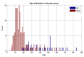
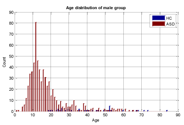
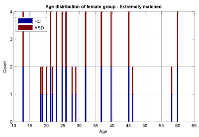
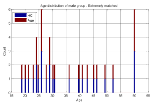
A key objective in applying machine learning algorithms in this study was to build a suitable training group from our dataset. Our dataset was comprised of 928 ASD subjects and 101 HC subjects which resulted in unbalanced data with the distribution shown in Figures 2 and 3 for both male and female subjects, therefore care should be taken in selecting appropriate training sets. We divided our patient data into two sets: one for training and the other for validation and testing. The training set should be large enough for the machine learning models to learn all the interdependencies among the variables. We carefully selected the appropriate size for training data to include the proper ratios of patients with respect to age, gender, and other relevant information. Construction of the proper training set takes time and entails an iterative process with feedback from experts. A number of experiments were conducted with different sets of features with our selected machine learning algorithms to finalize the training set and features.
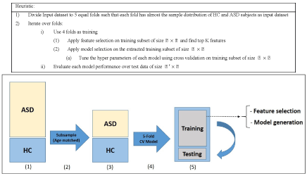
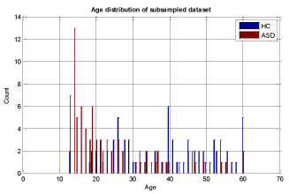
To ensure that the model building is complete with each selected machine learning algorithm, we used 5-fold cross validation and assessed the results with known labels (ground truth). In this cross validation phase, we divided the training set into 5 parts and iteratively used 4 out of 5 parts for training and then tested the models on the 5th part. The results of specificity and sensitivity for all 5 experiments were averaged to see how robust the current trained model is. This process is repeated by changing the training set and conducting experiments with different sets of features to achieve the best possible result. The details of our methodology are shown in Figure 3 and in the heuristic algorithm. The age distribution of sub-sampled datasets for stage (3) in Figure 3 is shown in Figures 5-7.
Results
Autism versus healthy controls
We conducted two sets of experiments – the first experiment is with subsampled data matching by age ranges and the second experiment is extremely matched by age and gender. In the first experiment we used the subsampling approach and obtained a subsample which has 168 instances. This dataset was achieved by removing all samples with missing values, mainly in ROI features and also limiting the age range of samples to those between 13-67 years old. In experiment 2, we applied the same sub-sampling method to extremely matched subjects with respect to age and gender. This dataset has 108 samples with 48 subjects of ASD and 48 subjects of HC group. The details of distribution of subjects based on age and gender are shown in Figures 3-7.
Experiment 1: Subsampling by age matching
In this experiment, we ran multiple classifiers on the dataset of 168 samples (84 healthy samples and 84 autism samples). We follow the steps of this framework to perform feature selection and model generation. For feature selection stage, we compared multiple approaches like LASSO, mRMR and PCA and achieved the most promising results by features selected with LASSO.
mRMR provides the feature set by requiring that features are maximally dissimilar to one another, for example, their mutual Euclidean distances are maximized, or their pair-wise correlations are minimized. These minimum redundancy criteria are supplemented by the usual maximum relevance criteria such as maximal mutual information with the target phenotypes. The benefits of this approach can be realized in two ways. (1) With the same number of features, we expect the mRMR feature set to be more representative of the target phenotypes, therefore leading to a better generalization property. (2) Equivalently, we can use a smaller mRMR feature set to effectively cover the same space as a larger conventional feature set [52]. The mRMR method is designed to work with discrete data and since we have continuous values in our dataset, before applying this method we need to discretize the data into multiple bins. This step is implemented by using Matlab built-in functions and we also use the available implementation of mRMR by the inventors of this method.
Lasso is a feature selection and also a regularization method that was originally introduced in the context of least squares. In this method, the sum of the absolute value of the regression coefficients are forced to be less than a fixed threshold value, which consequently leads to setting certain coefficients to zero. This approach is motivated by ridge regression, in which the coefficients sum of the squares is forced to be less than a fixed threshold value. Ridge regression shrinks the size of the large regression coefficients to reduce overfitting, but doesn’t perform covariate selection which consequently will not be able to build more interpretable models. Compared to mRMR, LASSO gave us more informative features in this experiment.
We also evaluated our designed model by the abstract features generated by PCA that leads to lower classification performance, compared to LASSO. Since we are mostly interested in finding highly correlated features representing the blood flow of 128 ROI regions, we stick to feature selection methods that promote sparsity as discussed earlier.
In this study we applied different approaches to find the best classification model that separates ASD patients from HC. We experimented with several well-known machine learning algorithms, including Random Forest (RF), Logistic Regression (LR) and Support Vector Machine (SVM). For all our experiments we used the scikit-learn package that implements all these algorithms .( http://scikit-learn.org/stable/index.html)
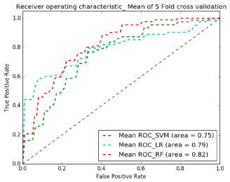
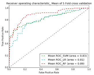
Figures 8 and 9 show receiver operating characteristic (ROC) plots which is a graphical plot that illustrates the performance of a binary classifier system and provides a visual overview for comparing the performance of classifiers. Table I shows the average specificity, sensitivity and accuracy across classifiers and demonstrates that the best classifier for both experiments is Random Forest.
Experiment 2: Subsampling by extreme subject matching based on age and gender
In experiment 2 we followed the same steps as in experiment 1 and simply replaced the input dataset with the extreme subsamples dataset that has 28 female subjects in each of the HC and ASD samples and 26 male subjects in each group that make a dataset of 108 subjects in total. This dataset classification performance is evaluated by the same classifiers in experiment 1. The classification performance results are shown in Tables 2A ,2B. Table 3 lists the top 12 ROI features in distinguishing ASD from controls:
Discussion
In the present study, ROI data from rest and on-task SPECT images were used to inform classification of ASD from HC using machine learning algorithms, attaining a maximum classification accuracy of 74.4% with Random Forest using subsampling methods with the top 12 features. This algorithm performed with a high level of accuracy on a robust dataset comprised of 168 with 84 ASD individuals and 84 HC, with a sensitivity and specificity respectively of 72% and 76% using only ROI features and 78% and 83% sensitivity and specificity by utilizing ROI features and age attributes.
Implementing several machine learning tools with varied feature sizes, we discovered that several algorithms reached an accuracy level to provide reliable diagnostic utility. SVM and Logistic Regression was also tested on the subsampled dataset with ROI regions and age, and resulted in accuracies of >76%. This work has not previously been performed with brain SPECT imaging data, so these results contribute to the growing body of literature in the neuroimaging field that have utilized pattern recognition with machine learning classification to improve distinguishing autism from typical developing subjects. Other methods include functional connectivity MRI [10,36,53-58], voxel based morphology [59], EEG [19,20,60,61] and diffusion tensor imaging studies [18].
Among the top most informative features identified using LASSO, we found involvement of regions implicated in ASD pathology, including regions of the cerebellum and vermis, anterior cingulate gyrus, amygdala, thalamus, frontal, and temporal lobes. The fact that both concentration and baseline SPECT scan ROIs were important in delineating between ASD and controls suggests that both scans may be useful in a clinical setting.
These regions are correlated with the core symptom domains of ASD including socio-communication deficits, impairments in cognition, language and repetitive/stereotyped movement and are consistent with previously described neuroimaging abnormalities. One of the most notable neuropathological hallmarks of ASD includes dysfunction of the cerebellar vermis, cortices and cerebro-cerebellar circuits [22,62,21]. This finding is consistent with structural and functional studies in MRI and SPECT, demonstrating the prevalence of cerebellar dysfunction in ASD. Such studies also demonstrated behavioral impairments with regard to motor control, language, social control, affective expression and exploratory attention [63]. The left anterior inferior temporal lobe was also important in our study in distinguishing between the two groups. Prior literature has shown the right temporal parietal junction is an associative region and has been shown to respond atypically in those with autism spectrum conditions [64]. This region has been implicated in the understanding of the “theory of mind,” [65] language, spatial cognition and attention that is implicated in the social-communication deficits observed in ASD. Furthermore, the amygdala was identified as a distinguishing feature. Limbic areas such as the amygdala are involved in emotional perception and regulation, and have been found to be enlarged in autistics [66]. The amygdala has been implicated in the socio-emotional impairments observed in autism, due to its widespread connectivity to cortical and subcortical structures [67]. Additional features identified include the frontal lobes, thalamus and posterior cingulate cortex which have been previously reported to show perfusion abnormalities with SPECT [41,42,68] and to correlate with the attentional dysfunction, the inability to modulate social behaviors, language and emotional processing deficits and the inability to perceive emotional expressions in autism. The fact that the left transverse temporal gyrus of Heschl on concentration SPECT was a distinguishing feature is intriguing, given the impaired auditory processing a prior MEG study found in autistic children [69]. Additional left-sided regions identified in our analysis may also related not only to the language functions of that hemisphere, but may also reflect the fact that most subjects in our sample were right-handed, thus denoting a left hemisphere dominance.
As ASD is increasingly prevalent and diagnosed in children, we wanted to ensure that age would not be a discriminating factor, therefore we applied our algorithms only to adults with ASD and the HC subjects and to an age matched range of 18-40 in both groups. In both of these experiments, our results were approximately equivalent when we used all the data in both groups.
There were several methodological challenges to address with this dataset to ensure best practices were followed for computational analysis using machine learning algorithms. Our first objective in designing this study was to obtain a large dataset of good quality with enough participants from each group for the model to learn from the training data. We then recognized that the high number of ROIs from the imaging data produced a dimensionality problem. We reduced the dimensionality by identifying the most important attributes that could reliably separate the two classes. We then had to address the imbalance in the number of subjects in the two classes by identifying which features to use and testing a number of experimental models with different algorithms to obtain the reported classification results. We evaluated each model carefully by setting aside some data for testing to avoid overfitting and to ensure generalizability of the model. And finally, further validation of the classifier was performed by testing our machine learning models on an independent test set containing both ASD and HC subjects. We performed these steps to assess the reliability of the data, because when predictive models show interpretable features that are reliable it offers the potential for diagnostic utility in a clinical setting.
This study had several strengths but also included limitations which need to be addressed for future studies. The strengths included neuroimaging data that was acquired both at rest and on-task from a well-validated and widely available functional imaging modality. This work was performed on a large sample size of ASD subjects obtained across multiple sites, and was measured with quantitative analysis using machine learning algorithims in which the classifier was validated on an independent data set. The first limitation was a retrospective analysis of existing data, so we did not have information on IQ or language ability to assess language delay. Therefore, this data must be interpreted across a broad range of intelligence and communication abilities. As the autism spectrum includes a wide range of intellectual ability, future work will include assessing IQ in order to perform more focused studies on differentiating low functioning, versus high functioning individuals from the HC group. Second, while diagnosis of ASD was established by meeting the DSM-IV criteria for autism as assessed by an expert clinician, inclusion of the Autism Diagnostic Interview-Revised or Autism Diagnostic Observation Schedule would address the level of functionality of the patients. And finally, future work will not only include the HC group, but will also include individuals with mood disorders including attention deficit hyperactivity disorder (ADHD), anxiety and obsessive compulsive disorder. Studies with a HC allow for understanding the neurobiological underpinnings of the ASD, but symptoms of autism and psychiatric disorders such as ADHD often co-occur [70], and it will be important to explore how machine learning approaches can be used to understand the neurobiological differences between autism and co-morbid disorders, as this is what occurs in a real-world clinical setting.
The clinical relevance of this work is its identification of specific brain regions on perfusion SPECT neuroimaging that diagnostically distinguish autism from controls. Because these findings were obtained from a large database, there exists a foundation for development of computer algorithms for individualized prediction of diagnosis. For example, a single patient scan can be inputted into a machine learning program and then matched to a brain SPECT scan database of pre-existing controls and patient scans such as with autism. The patient’s scan could then be matched to either a patient or control group based on quantified imaging characteristics in combinations of regions specific for various disorders from autism to Alzheimer’s to TBI.
To our knowledge this is the first brain SPECT imaging study demonstrating the use of machine learning methods to predict ASD from a HC. These results add to the growing body of literature validating the use of machine learning approaches with functional neuroimaging data to improve prediction and classification of individuals with psychiatric disorders like autism. Given the heterogeneity of ASD, this approach has important implications in the clinical setting in both the diagnosis, intervention and monitoring of treatment outcomes.
References
- Christensen DL, Baio J, Van Naarden Braun K., et al. (2016) Prevalence and characteristics of autism spectrum disorder among children aged 8 years autism and Developmental Disabilities Monitoring Network, 11 sites, United States, 2012. MMWR Surveill 65: 1 -23.
- Geschwind DH, Levitt P (2007) Autism spectrum disorders: developmental disconnection syndromes. Curr Opin Neurobiol 17: 103-111. [Crossref]
- Lord C, Rutter M, A Le Couteur (1994) Autism Diagnostic Interview-Revised: a revised version of a diagnostic interview for caregivers of individuals with possible pervasive developmental disorders. J Autism Dev Disord 24: 659-685. [Crossref]
- Gotham K, Risi S, Pickles A, Lord C (2007) The Autism Diagnostic Observation Schedule: revised algorithms for improved diagnostic validity. J Autism Dev Disord 37: 613-627. [Crossref]
- Levy SE, Mandell DS, Schultz RT (2009) Autism. Lancet 374: 1627-1638. [Crossref]
- Wiggins LD, Baio J, Rice C (2006) Examination of the time between first evaluation and first autism spectrum diagnosis in a population-based sample. J Dev Behav Pediatr 27: S79-87. [Crossref]
- Retico A, Tosetti M, Muratori F, Calderoni S (2014) Neuroimaging-based methods for autism identification: a possible translational application? Funct Neurol 29: 231-239. [Crossref]
- Levman J, Takahashi E (2015) Multivariate analyses applied to fetal, neonatal and pediatric MRI of neurodevelopmental disorders. Neuroimage Clin 9: 532-544. [Crossref]
- Jin, Y., C. Y. Wee, F. Shi, K. H. Thung, D. Ni, P. T. Yap and D. Shen (2015). "Identification of infants at high-risk for autism spectrum disorder using multiparameter multiscale white matter connectivity networks." Hum Brain Mapp 36(12): 4880-4896.
- Plitt M, Barnes KA, Martin A (2015) Functional connectivity classification of autism identifies highly predictive brain features but falls short of biomarker standards. Neuroimage Clin 7: 359-366. [Crossref]
- Ecker C, Rocha-Rego V, Johnston P, Mourao-Miranda J, Marquand A, et al. (2010) Investigating the predictive value of whole-brain structural MR scans in autism: a pattern classification approach. Neuroimage 49: 44-56. [Crossref]
- Sato JR, Hoexter MQ, Oliveira PP, Brammer MJ, Consortium MA, et al. (2013) Inter-regional cortical thickness correlations are associated with autistic symptoms: a machine-learning approach. J Psychiatr Res 47: 453-459. [Crossref]
- Gori I, Alessia G, Filippo M, Irene S, Piernicola O, et al. (2015) Gray Matter Alterations in Young Children with Autism Spectrum Disorders: Comparing Morphometry at the Voxel and Regional Level. J Neuroimaging 25: 866-874. [Crossref]
- Anderson JS, Nielsen JA, Froehlich AL, DuBray MB, Druzgal TL, et al. (2011) Functional connectivity magnetic resonance imaging classification of autism. Brain 134: 3742-3754. [Crossref]
- Nielsen JA, Zielinski BA, Fletcher PT, Alexander AL, Lange N, et al. (2013) Multisite functional connectivity MRI classification of autism: ABIDE results. Front Hum Neurosci 7: 599. [Crossref]
- Uddin LQ, Supekar K, Lynch CJ, Khouzam A, Phillips J, et al. (2013) Salience network-based classification and prediction of symptom severity in children with autism. JAMA Psychiatry 70: 869-879. [Crossref]
- Lange N, Dubray MB, Lee JE, Froimowitz MP, Froehlich A, et al. (2010) Atypical diffusion tensor hemispheric asymmetry in autism. Autism Res 3: 350-358. [Crossref]
- Ingalhalikar M, Parker D, Bloy L, Roberts TP, Verma R (2011) Diffusion based abnormality markers of pathology: toward learned diagnostic prediction of ASD. Neuroimage 57: 918-927. [Crossref]
- Bosl W, Tierney A, Tager-Flusberg H, Nelson C (2011) EEG complexity as a biomarker for autism spectrum disorder risk. BMC Med 9: 18. [Crossref]
- Duffy FH, Als H (2012) A stable pattern of EEG spectral coherence distinguishes children with autism from neuro-typical controls - a large case control study. BMC Med 10: 64. [Crossref]
- Hampson DR, Blatt GJ (2015) Autism spectrum disorders and neuropathology of the cerebellum. Front Neurosci 9: 420. [Crossref]
- Courchesne E, Yeung-Courchesne R, Press GA, Hesselink JR, Jernigan TL (1988) Hypoplasia of cerebellar vermal lobules VI and VII in autism. N Engl J Med 318: 1349-1354. [Crossref]
- Yang X, Si T, Gong Q, Qiu L, Jia Z, et al. (2016) Brain gray matter alterations and associated demographic profiles in adults with autism spectrum disorder: A meta-analysis of voxel-based morphometry studies. Aust N Z J Psychiatry 50: 741-753. [Crossref]
- Sparks BF, Friedman SD, Shaw DW, Aylward EH, Echelard D, et al. (2002) Brain structural abnormalities in young children with autism spectrum disorder. Neurology 59: 184-192. [Crossref]
- Herrington JD, Miller J, Pandey J, Schultz RT (2016) Anxiety and Social Deficits Have Distinct Relationships with Amygdala Function in Autism Spectrum Disorder. Soc Cogn Affect Neurosci 11: 907-914. [Crossref]
- Rausch A, Zhang W, Haak KV, Mennes M, Hermans EJ, et al. (2016) Altered functional connectivity of the amygdaloid input nuclei in adolescents and young adults with autism spectrum disorder: a resting state fMRI study. Mol Autism 7: 13. [Crossref]
- Barnea-Goraly N, Frazier TW, Piacenza L, Minshew NJ, Keshavan MS, et al. (2014) A preliminary longitudinal volumetric MRI study of amygdala and hippocampal volumes in autism. Prog Neuropsychopharmacol Biol Psychiatry 48: 124-128. [Crossref]
- Sussman D, Leung RC1, Vogan VM1, Lee W1, Trelle S1, et al. (2015) The autism puzzle: Diffuse but not pervasive neuroanatomical abnormalities in children with ASD. Neuroimage Clin 8: 170-179. [Crossref]
- Foster NE, Doyle-Thomas KA, Tryfon A, Ouimet T, Anagnostou E, et al.(2015) Structural Gray Matter Differences During Childhood Development in Autism Spectrum Disorder: A Multimetric Approach. Pediatr Neurol 53: 350-359. [Crossref]
- Nair A, Carper RA, Abbott AE, Chen CP, Solders S, et al. (2015) Regional specificity of aberrant thalamocortical connectivity in autism. Hum Brain Mapp 36: 4497-4511. [Crossref]
- Solso S, Xu R, Proudfoot J, Hagler DJ, Campbell K, et al. (2015) Diffusion Tensor Imaging Provides Evidence of Possible Axonal Overconnectivity in Frontal Lobes in Autism Spectrum Disorder Toddlers. Biol Psychiatry 79: 676-684. [Crossref]
- Abell F, Krams M, Ashburner J, Passingham R, Friston K, et al. (1999) The neuroanatomy of autism: a voxel-based whole brain analysis of structural scans. Neuroreport 10: 1647-1651. [Crossref]
- Sato W, Kubota Y, Kochiyama T, Uono S, Yoshimura S, et al. (2014) Increased putamen volume in adults with autism spectrum disorder. Front Hum Neurosci 8: 957. [Crossref]
- Jiao Y, Chen R, Ke X, Chu K, Lu Z, et al. (2010) Predictive models of autism spectrum disorder based on brain regional cortical thickness. Neuroimage 50: 589-599. [Crossref]
- Bloy L, Ingalhalikar M, Eavani H, Roberts TP, Schultz RT et al. (2011) HARDI based pattern classifiers for the identification of white matter pathologies. Med Image Comput Comput Assist Interv 14: 234-241. [Crossref]
- Chen CP, Keown CL, Jahedi A, Nair A, Pflieger ME, et al. (2015) Diagnostic classification of intrinsic functional connectivity highlights somatosensory, default mode, and visual regions in autism. Neuroimage Clin 8: 238-245. [Crossref]
- Zurcher NR, Bhanot A, McDougle CJ, Hooker JM (2015) A systematic review of molecular imaging (PET and SPECT) in autism spectrum disorder: current state and future research opportunities. Neurosci Biobehav Rev 52: 56-73. [Crossref]
- Carina Gillberg I, Bjure J, Uvebrant P, Vestergren E, Gillberg C (1993) SPECT (Single Photon Emission Computed Tomography) in 31 children and adolescents with autism and autistic-like conditions. Eur Child Adolesc Psychiatry 2: 50-59. [Crossref]
- Kaya M, Karasalihoglu S, Ustun F, Gultekin A, Cermik TF, et al. (2002) The relationship between 99mTc-HMPAO brain SPECT and the scores of real life rating scale in autistic children. Brain Dev 24: 77-81. [Crossref]
- Wilcox J, Tsuang MT, Ledger E, Algeo J, Schnurr T (2002) Brain perfusion in autism varies with age. Neuropsychobiology 46: 13-16. [Crossref]
- Ito H, Mori K, Hashimoto T, Miyazaki M, Hori A, et al. (2005) Findings of brain 99mTc-ECD SPECT in high-functioning autism--3-dimensional stereotactic ROI template analysis of brain SPECT. J Med Invest 52: 49-56. [Crossref]
- Sasaki M, Nakagawa E, Sugai K, Shimizu Y, Hattori A, et al. (2010) Brain perfusion SPECT and EEG findings in children with autism spectrum disorders and medically intractable epilepsy. Brain Dev 32: 776-782. [Crossref]
- Yang WH, Jing J, Xiu LJ, Cheng MH, Wang X, et al. (2011) Regional cerebral blood flow in children with autism spectrum disorders: a quantitative (9)(9)mTc-ECD brain SPECT study with statistical parametric mapping evaluation. Chin Med J (Engl) 124: 1362-1366.
- Amen DG, Hanks C, Prunella J (2008) Preliminary evidence differentiating ADHD using brain SPECT imaging in older patients. J Psychoactive Drugs 40: 139-146. [Crossref]
- Amen DG, Hanks C, Prunella J (2008) Predicting positive and negative treatment responses to stimulants with brain SPECT imaging. J Psychoactive Drugs 40: 131-138. [Crossref]
- Chang W, Henkin RE, Buddemeyer E (1984) The sources of overestimation in the quantification by SPECT of uptakes in a myocardial phantom: concise communication. J Nucl Med 25: 788-791. [Crossref]
- Tzourio-Mazoyer N, Landeau B, Papathanassiou D, Crivello F, Etard O, et al. (2002) Automated anatomical labeling of activations in SPM using a macroscopic anatomical parcellation of the MNI MRI single-subject brain. Neuroimage 15: 273-289. [Crossref]
- Rothenberg TJ, Fisher FM, Tilanus CB (1964) A note on the estimation of the location parameters of the Cauchy distribution. J Amer Statistic Assoc 61: 852-855. [Crossref]
- Raji CA, Tarzwell R, Pavel D, Schneider H, Uszler M, et al. (2014) Clinical utility of SPECT neuroimaging in the diagnosis and treatment of traumatic brain injury: a systematic review. PLoS One 9: e91088. [Crossref]
- Foster KR, Koprowski R, Skufca JD (2014) Machine learning, medical diagnosis, and biomedical engineering research - commentary. Biomed Eng Online 13: 94. [Crossref]
- Tibshirani R (1996) Regression Shrinkage and Selection via the lasso. Journal of the Royal Statistical Society 58: 267–88. [Crossref]
- Goldani AA, Downs SR, Widjaja F, Lawton B, Hendren RL (2014) Biomarkers in autism. Front Psychiatry 5: 100. [Crossref]
- Murdaugh DL, Shinkareva SV, Deshpande HR, Wang J, Pennick MR, et al. (2012) Differential deactivation during mentalizing and classification of autism based on default mode network connectivity. PLoS One 7: e50064. [Crossref]
- Wang H, Chen C, Fushing H(2012). Extracting multiscale pattern information of fMRI based functional brain connectivity with application on classification of autism spectrum disorders. PLoS One 7: e45502. [Crossref]
- Deshpande G, Libero LE, Sreenivasan KR, Deshpande HD, Kana RK (2013) Identification of neural connectivity signatures of autism using machine learning. Front Hum Neurosci 7: 670. [Crossref]
- Marcel AJ, Vladimir LC, Augusto B, Timothy AK, Tom MM (2014) Identifying autism from neural representations of social interactions: neurocognitive markers of autism. PLoS One 9: e113879. [Crossref]
- Zhou Y, Yu F, Duong T (2014) Multiparametric MRI characterization and prediction in autism spectrum disorder using graph theory and machine learning. PLoS One 9: e90405. [Crossref]
- Plitt M, Barnes KA, Wallace GL, Kenworthy L, Martin A (2015) Resting-state functional connectivity predicts longitudinal change in autistic traits and adaptive functioning in autism. Proc Natl Acad Sci U S A 112: E6699-6706. [Crossref]
- Gori I, Giuliano A, et al. (2015) Gray Matter Alterations in Young Children with Autism Spectrum Disorders: Comparing Morphometry at the Voxel and Regional Level. J Neuroimaging 25: 866-874. [Crossref]
- Stahl D, Pickles A, Elsabbagh M, Johnson MH; BASIS Team (2012) Novel machine learning methods for ERP analysis: a validation from research on infants at risk for autism. Dev Neuropsychol 37: 274-298. [Crossref]
- Jamal W, Das S, Oprescu IA, Maharatna K, Apicella F, et al. (2014) Classification of autism spectrum disorder using supervised learning of brain connectivity measures extracted from synchrostates. J Neural Eng 11: 046019. [Crossref]
- D'Mello AM, Stoodley CJ (2015) Cerebro-cerebellar circuits in autism spectrum disorder. Front Neurosci 9: 408. [Crossref]
- Trevarthen C, Delafield-Butt JT (2013) Autism as a developmental disorder in intentional movement and affective engagement. Front Integr Neurosci 7: 49. [Crossref]
- Lombardo MV, Chakrabarti B, Bullmore ET, Consortium MA, Baron-Cohen S (2011) "Specialization of right temporo-parietal junction for mentalizing and its relation to social impairments in autism." Neuroimage 56: 1832-1838. [Crossref]
- Li W, Mai X, Liu C (2014) The default mode network and social understanding of others: what do brain connectivity studies tell us. Front Hum Neurosci 8: 74. [Crossref]
- Groen W, Teluij M, Buitelaar J, Tendolkar I (2010) Amygdala and hippocampus enlargement during adolescence in autism. J Am Acad Child Adolesc Psychiatry 49: 552-560. [Crossref]
- Baron-Cohen S, Ring HA, Bullmore ET, Wheelwright S, Ashwin C, et al. (2000) The amygdala theory of autism. Neurosci Biobehav Rev 24: 355-364. [Crossref]
- Ohnishi T, Matsuda H, Hashimoto T, Kunihiro T, Nishikawa M, et al. (2000) Abnormal regional cerebral blood flow in childhood autism. Brain 123: 1838-1844. [Crossref]
- Brennan JR, Wagley N, Kovelman L, Bowyer SM, Richard AE, et al. (2016). Magnetoencephalography shows atypical sensitivity to linguistic sound sequences in autism spectrum disorder. Neuroreport 27: 982-986. [Crossref]
- Leitner Y (2014) The co-occurrence of autism and attention deficit hyperactivity disorder in children - what do we know? Front Hum Neurosci 8: 268. [Crossref]
2021 Copyright OAT. All rights reserv


